JPK Nanowizard 3 Bioscience AFM
Short manual
This is a short from manual to get started with the JPK Nanowizard
Bioscience system. The AFM head is mounted on top of an inverted
optical microscope. The microscope has two illumination scources which
can be used concurrently with the AFM scanning.
The most sensitive part is the afm tip holder and of course the tip
itself. Therefore this instruction start with how to handel the tip
holders and how to mount a tip.
|
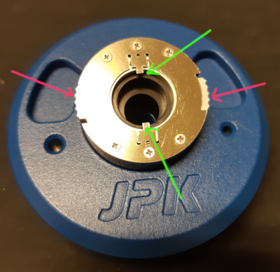
This is the mounting tool for the tip holder. It has a circular
opening for the tip holder, and two locking tabs at the top and
bottom (green arrows). The locking tabs can be released or
locked by turning
the outer white sliders (red
arrows) clockwise or anti clockwise.
|
|
|
|
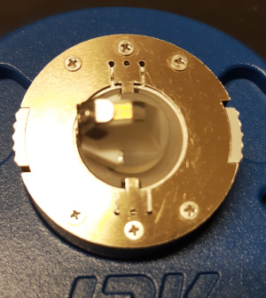
Here the tip holder is inserted into the mounting tool. There
are two cutouts in the holder that fits the locking tabs.
|
The tip holder is rotated 90 degrees and the white sliders are
moved so the locking tabs fixate the tip holder.
|
|
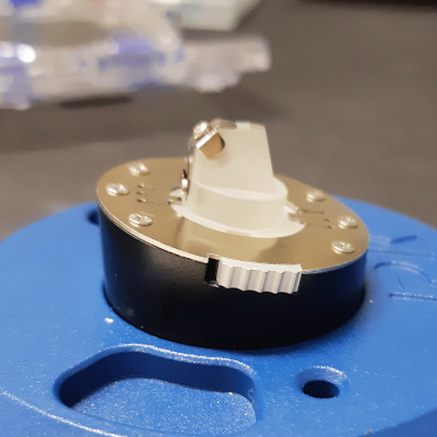
Side view of the mounting tool with the tip holder. Please note
that the mounting tool is slanted to compensate for the slanted
bottom surface of the tip holder.
Rotate the tip holder in the
correct direction prior to locking.
In this way the top surface
of the tip holder become horisontal, making it possible to mount
the tip without it falling off.
|
|
|
|
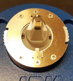
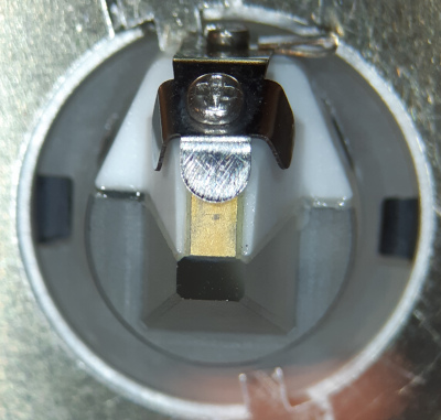
Top view of tip holder. This is the variant of tip holder that
has a piezo shaker at the top. The piezo crystal (light yellow)
is mounted on a
plastic part which is glued to the glass part of the tip holder.
At the top in th image is the clamp with its fastening
screw. The screw should never be overtightened, there is a high
risk of deforming the clamp and even break the holder.
The glass part is of high optical quality, the glass surface
directly below the piezo in the image must be handled with
care, not to be scratched.
|
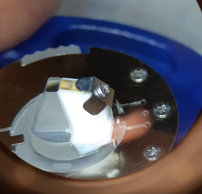
Side view of the tip holder in the mounting tool. The clamp with
its screw, the piezo shaker is clearly visible. Placing the
piezo shaker directly in contact with the cantilever is more
efficient than shaking the whole glass body.
|
Pic of holder with cantilever.
The Microscope X-Y Stage controller has to be powered on before
starting the software!
The software
|
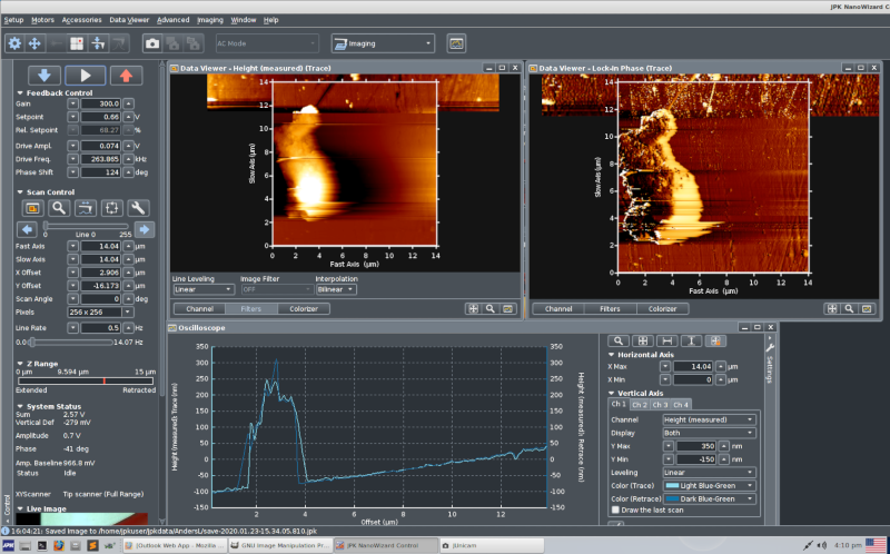
Overview of software, left half. There are two screens, this is
the left screen.
At the top, below the dropdown menues, are function buttons
for different parts of the setup and scanning.
Below are the controls for engaging, scanning and retraction.
In the center are two data viewers showing height and phase
in AC-mode (tapping mode).
At the bottom is an "oscilloscope" showing trace and
retrace of the height signal.
|
|
The left screen usually shows this, although screen layout is of
course fully configurable.
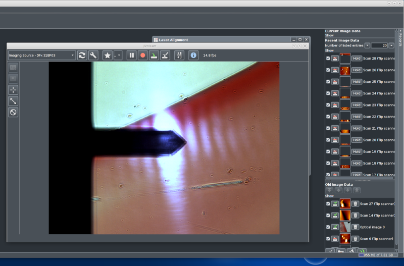
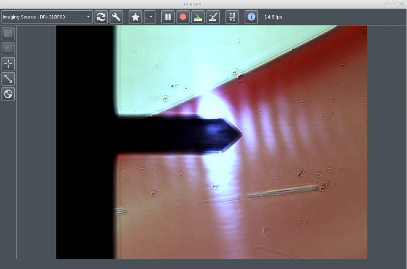
The CCD camera window showing a live video image of the
sample. Here is ordinary transmission illumination (white
light). The sample is a microscope object slide with some pen
markings. The cantilever is clearly visible, it is quite near
the top surface of the glass slide, therefore it is in good
focus.
The white oblong dots are the laser spot (and its secondary
maxima) that is positioned on the back of the cantilever.
Behind the camera window is the laser alignment window, it
will be shown separately below.
To the right is a stack of image data collected. These are
kept in memory, and only saved to disk by user
interaction. When the software is exited the user is prompted
for saving data that is still only in RAM.
|
WARNING!!!
When the X-Y stage control and Joystick box are used, please note that
when the stage control is Enabled, almost everything else is
disabled. You cannot change scanning mode, not move leg motors, not
engage.
Click once on Engage button to activate, click again to de-activate.
 The stage control window is opened with this
func. button
The stage control window is opened with this
func. button  .
The stage control is described in more detail below.
.
The stage control is described in more detail below.
When the cantilever has been mounted on the tip holder and the holder
mounted on the scanhead, the scanhead is placed on the microscope
table. Each leg of the scan head fits in a separate place of the
table, a flat, a groove and a conical hole. This way the scan head
is positioned in a reproducible way on the stage.
The scan head must have its legs so much extended so there is now
risk of damaging the cantilever. This is usually ensured by the
extension from a previous retraction at the end of a scanning
session.
Each separate window is opened by a corresponding function button.
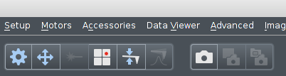
From left to right:
- Z Motor control
- X-Y Microscope Stage control
- Laser on/Off
- Laser Alignment
- Cantilever Stiffness Calibration
- Tuning cantilever
- Camera window
- Save camera image????
- Save camera image????
|
It is good to always open the Camera Control window first in order
to keep track of where the cantilever is.
This is done by
clicking 
Initially the sample should NOT be mounted.
When setting up the cantilever, adjusting laser spot, etc. it is much
easier without any sample slide between the microscope objective and
the cantilever.
The microscope should be
focused on the cantilever. This will be a great help when aligning
the laser spot onto the backside of the cantilever (see further
below).
The CCD camera window showing a live video image of the
sample. Here is ordinary transmission illumination (white
light). The sample is a microscope object slide with some pen
markings. The cantilever is clearly visible, it is quite near
the top surface of the glass slide, therefore it is in good
focus.
The white oblong dots are the laser spot (and its secondary
maxima) that is positioned on the back of the cantilever.
|
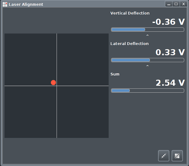
Laser Alignment is opened by

|
First the Sum signal should be maximised by aiming the laser
spot as well as possible on the back of ther cantilever. The
camera image is of great help here, since the laser spot is
visible in the camera image.
The illumination intensity may have
to be balanced against the laser spot intensity in order to make
it visible in the camera image.
After that the Vertical and Lateral deflections are minimised
using the knobs on the scan head.
|
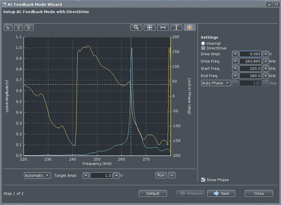
The resonance frequency has to be found for the current cantilever
mounted, window is opened by
clicking 
|
Frequency sweep displayed in oscilloscope-like window.
The sweep can be zoomed using the pointer and scroll wheel.
When the resonance peak is filling most of the display, the
drive frequency and amplitude can be set by pointing and
clicking in the graph. Amplitude should usually be around 0.7 V.
The range
of the sweep can also be set by the fields at the upper right,
"Start Freq." and "End Freq.".
|
Now it is time to mount the sample. Lower the microscope objective
much downward. The objective has been quite high up, probably above
the surface of the microscope stage, this in order to be able to focus
on the cantilever.
Motor Control window is opened by
clicking 
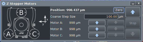
At the right are Up and Down arrows to step all three legs
equally to approach or retract form the sample surface. The step
size can be set, 100 ‐ 500 µm are common values.
When approaching the surface the optical microscope should be
used to check how close to the surface the cantilever is. This
to avoid crashing into the surface, breaking the cantilever.
The Zero button is for setting the current position to zero.
The three stepper motors can be controlled separately by the
center arrows, although this is rarely used.
|
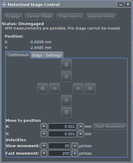
There is a motor controlled microscope stage for movement in the X-Y
directions.
The stage motor controller has to be powered on before starting
the software
The X-Y stage software control window is opened by
clicking
|
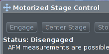
At the top are four function buttons. The "Engage" button
has to be clicked in order for the stage to work at all.
Please note that this will disable almost ALL other parts of the
software! Press "Engage" again to disable and get the
other parts of the software to work again.
The
"Joystick Mode" has to be clicked in order to activate the
joystick on the controller.
At the top of the joystick on the controller there is a push button
for high and low
speed. This button is a toggle button, one push for high speed, one
more push: back to low speed.
|
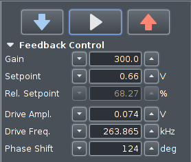
Scan Control / Feedback Control
This part of the software is always present on the screen,
it is located at the top left of the screen.
It does not have a function button to open it.
|
|
|
In order to do the approach and engage the cantilever to the sample
surface, a slow approach is done. This is started by clicking the blue
down arrow.
The approach will happen in a saw-tooth like movement. The Z-piezo for the
tip will extend slowly for 15 µm. If the surface is not reached
the Z-piezo will retract 15 µm and the three leg motors will
lower the scan head 15 µm very fast. Then the process starts
over again.
The value for Gain is usually correctly set up. The
values for Setpoint, Drive Ampl. and Drive Freq. are taken from the
tuning window.
When the engage has been completed, the cantilever tip is resting on,
or is extremely near the surface.
In order for the actual scanning of the surface to start you have to
click the white left-pointing arrow, center top button.
|
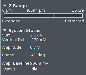
During the approach (engage), the Z position for the tip is displayed
here. It will be a cyclic process, the piezo will slowly extend downwards
from zero to 15 µm, then retract at the same time as the
leg motors quickly
move the scan head down 15 µm.
Here is also shown the Z-range used during scanning of the sample
surface.
|
|
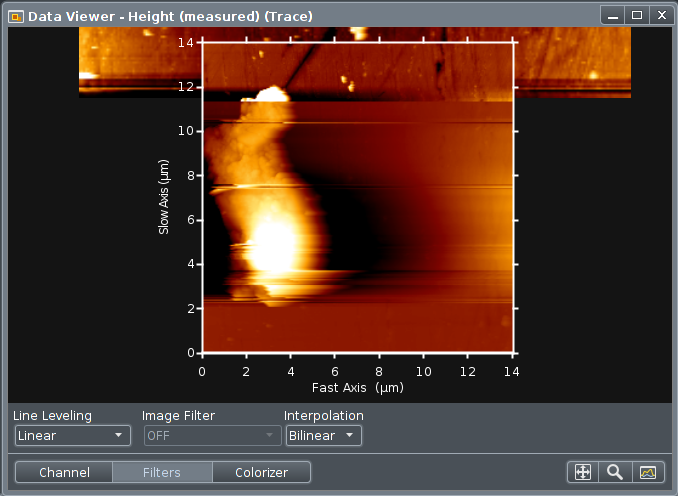
During scanning the sample surface is displayed in a "Data
Viewer". This window have several controls for which signal
to be displayed, the levelling etc.
The viewable area can be zoomed using the pointer and scroll
wheel. A new scan area can be drawn using pointer and drag
left button.
Using a drop down menu item under "Accessories????"
it is possible to acquire and calibrate an optical image from
the microscope as a coarse map to find interesting areas for
detailed AFM/SPM scanning. This optical image will be shown
underneath the areas scanned with the afm.
|
|
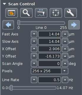
The size of the scan area can be set here, as well as offsets,
rotation (scan angle), size of image, and scan speed (line rate).
|
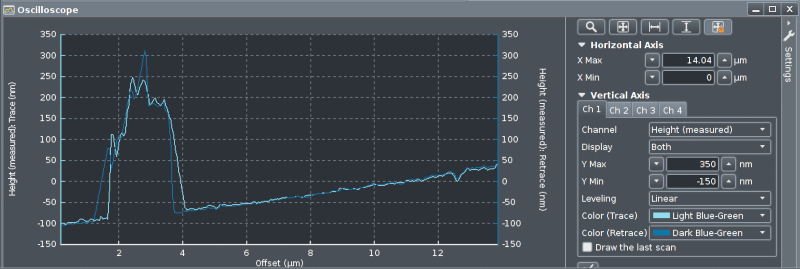
During scanning the traces can be displayed in an oscilloscope like
window, this is opened by clicking

|
Here the "Height" signal is displayed, both trace and
retrace. To the right are numerous controls for how the signals
will be displayed. Up to four channels can be displayed, and
here "Levelling" is set to "Linear" to get
rid of extra tilt on the sample surface.
Using the shape of the "Height" signal Gain and
Setpoint settings can be adjusted for best surface tracking.
|
|
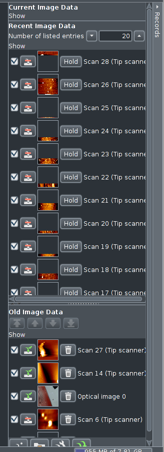
All scans are collected in system RAM (volatile memory). The are
displayed in a stack like manner. In the upper part there are data
sets that are only residing in RAM, not yet stored to disk. The little
button after the tick mark indicates this by a red dash over a small
bent arrow pointing to a disk icon.
In the lower part, "Old Image Data", there are data sets
stored to disk, the button shows a green tick mark next to a green
bent arrow pointing to the disk icon.
It is recommended to save data regularly, either by clicking
 for an individual
important dataset, or save all datasets to disk by clicking the
double green arrow button at the bottom (partly hidden)
for an individual
important dataset, or save all datasets to disk by clicking the
double green arrow button at the bottom (partly hidden)
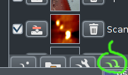
Clicking the "Hold" button will transfer data sets to
"Old Image Data". Data sets can be deleted from disk
(permanently) by clicking the
trashcan icon.
Upon exit of the software, the user is prompted to save all unsaved
data sets still in volatile memory.
|
|
How to start ImAFM software
- Start JPK controller
- Start JPK Software
- Set it to "Contact Mode"
- Start ImAFM software (desktop icon)
- In JPK software: Advanced ‐ Open Script
- Double-click "ImAFMSetup.py", this will add a button "ImAFM" along
the other function buttons in the JPK software
- Click on "ImAFM" button, opens a small window.
-
Click "Setup" in this small window, will enable trigger signals
necessary for ImAFM software.
Use
an optical microscope image as backgound map
Anders Liljeborg
Albanova Nanolab, KTH, SU.