While the NanoScope analysis software includes many useful routines, sometimes one might wish to import a force volume image into third party software—a spreadsheet program or an image processing system. The following discussion explains how to extract data from a saved (captured) force volume image.
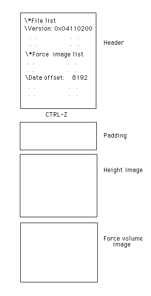
Like all NanoScope image files, the force volume image file has two parts: a header, and one or more images (see Figure 1). The header contains a series of lists, each of which contains a number of parameters. There is a list for the microscope, for the piezoelectric actuator, for the images, and for the force curves. Basically, every parameter under operator control is written to some line in a list in the header. This information, when combined with the data stored in the images, can be used to reconstruct the original images.
Figure 1: Force Volume Data File Structure.
The end of the header is flagged with a CTRL-Z character (ASCII 26). Different types of files have different length headers, but they all end with the CTRL-Z. There is a block of padding (random) data between the header and the actual images. The height image (Channel 1) is first, followed by the force volume image. All the image data is saved by the NanoScope software with 16 bits per pixel, (i.e., in 2’s complement notation for negative numbers with the least significant byte (LSB) in “little endian” form).
The height image data begins at byte 8192. It is a two dimensional array of data. The section explains how to reconstruct the image from information in the header.
The force volume data is stored as a series of force curves. Depending on the resolution of the height image, the starting byte will vary. The start position of the force volume data can be found in the Data offset line of the Ciao Force List, designated as:
\*Ciao Force List
. .
. .
\Data offset:
Regardless of which is displayed during data collection, both the retract and extend portions of the force curve are written to disk. The force curve data set is a linear array of deflection values. The first half of the array is the retracting portion of the curve; the second half is the extending portion. Both Z position and deflection values need to be scaled based on header values.
The force curves which make up the force volume image are saved in column major format. For example, if Number of samples is 256 and Force per line is 32, then there are 32 x 32 = 1024 force curves, each with 512 (retract and extend) deflection values. The force curves are ordered such that the first 32 form the first row of the image, the second 32 the next row, etcetera.
Only the deflection values of the force curves are saved to the file. The corresponding Z-position values are calculated from information in the header:
z = index *440.0 * zsens * zscansize / (65536.0 * samples)
where index = the index in the Z direction, 0-511, of a deflection value
zsens = \Z sensitivity
zscansize = \*Force image list\Scan Size
samples = \*Force image list\Samps/line
Deflection values are scaled according to the following formula:
deflscaled = deflraw* (20.0 /dsens) / 65536.0
where deflraw = the raw, integer values from the file.
dsens = \Detect sens.
Once the force volume data has been extracted from the file, it can be processed and analyzed by third party software such as RSI’s IDL, NIH Image, or Adobe Photoshop.
Third party graphics software is needed to construct a composite figure of several slices or representative force curves pictured along with the height image, for example. The images (heights or slices) and force curves need to be saved/exported individually and then loaded into the third party software.
| www.bruker.com | Bruker Corporation |
| www.brukerafmprobes.com | 112 Robin Hill Rd. |
| nanoscaleworld.bruker-axs.com/nanoscaleworld/ | Santa Barbara, CA 93117 |
| Customer Support: (800) 873-9750 | |
| Copyright 2010, 2011. All Rights Reserved. |