Calibrate the Spring Constant Using Thermal Tuning

NOTE: Bruker recommends Thermal Tune included in NanoScope software for probes with spring constants less than or equal to 1 N/m. Other methods (Sader1, added mass, vibrometer, pre-calibrated probes) are recommended for probes with higher spring constants.These techniques are reviewed in detail in Bruker Application Note 94: Practical Advice on the Determination of Cantilever Spring Constants.

Ensure that the probe is withdrawn adequately from the sample before activating Thermal Tune. The probe should not interact with the sample during its self excitation under ambient conditions.

Click Calibrate > Thermal Tune or the Thermal Tune icon in the NanoScope tool bar (shown).

Select a frequency range that includes the resonant frequency of the cantilever (see Figure 1). Stiff cantilevers may require the 5–2000 kHz range.

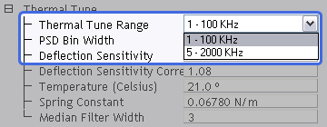
Figure 1: Select Thermal Tune Frequency Range

Click Acquire Data in the Thermal Tune panel, shown in Figure 2.

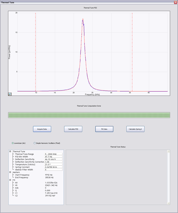
Figure 2: The Thermal Tune panel

The microscope will acquire data for about 30 seconds.
Zoom in on the region around the peak.
Click either the Lorentzian (Air) or Simple Harmonic Oscillator (Fluid) button to select a Lorentzian or a simple harmonic oscillator model, respectively, of the PSD to be least squares fit to the data.

NOTE: The equations used to fit the filtered data are:

Lorentzian, for use in air:

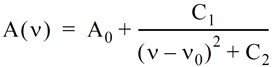
where:

A(ν) is the amplitude as a function of frequency, ν
A0 is the baseline amplitude
ν0 is the center frequency of the resonant peak
C1 is a Lorentzian fit parameter
C2 is a Lorentzian fit parameter

Simple Harmonic Oscillator, for use in fluid

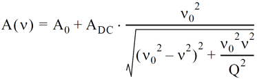
where:

A(ν) is the amplitude as a function of frequency, ν
A0 is the baseline amplitude
ADC is the amplitude at DC (zero frequency)
ν0 is the center frequency of the resonant peak
Q is the quality factor

Adjust the Median Filter Width, shown in Figure 3, to remove individual (narrow) spikes. This replaces a data point with the median of the surrounding n (n =3, 5, 7) data points.

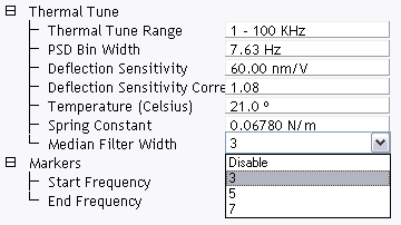
Figure 3: Median filter width

Adjust the PSD Bin Width to reduce the noise by averaging.
Drag markers in from the left and/or right plot edges to bracket the bandwidth over which the fit is to be performed. See Figure 2.
Click Fit Data. The curve fit, in red, is displayed along with the acquired data. If necessary, adjust the marker positions and fit the data again to obtain the best fit at the thermal peak.
Enter the cantilever Temperature.
Click Calculate Spring K.
You will be asked whether you want to accept the calculated value of the spring constant, k (see Figure 4). Clicking OK copies the calculated spring constant to the Spring Constant window in the Cantilever Parameters window.

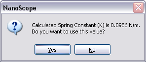
Figure 4: Spring Constant Calculation Result

www.bruker.com

Bruker Corporation

www.brukerafmprobes.com

112 Robin Hill Rd.

nanoscaleworld.bruker-axs.com/nanoscaleworld/

Santa Barbara, CA 93117

Customer Support: (800) 873-9750

	Ensure that the probe is withdrawn adequately from the sample before activating Thermal Tune. The probe should not interact with the sample during its self excitation under ambient conditions.
	Click Calibrate > Thermal Tune or the Thermal Tune icon in the NanoScope tool bar (shown).
	Select a frequency range that includes the resonant frequency of the cantilever (see Figure 1). Stiff cantilevers may require the 5–2000 kHz range.