You are here: NanoScope Software User Guide > Offline Commands > Analysis Functions > Depth

Depth

To analyze the depth of features you have numerous choices which measure the height difference between two dominant features that occur at distinct heights. Depth analysis was primarily designed for automatically comparing feature depths at two similar sample sites (e.g., when analyzing etch depths on large numbers of identical silicon wafers).

Theory

The Depth command accumulates depth data within a specified area, applies a Gaussian low-pass filter to the data to remove noise, then obtains depth comparisons between two dominant features.

Although this method of depth analysis does not substitute for direct, cross-sectioning of the sample, it affords a means for comparing feature depth between two similar sites in a consistent, statistical manner.

The Depth window includes a top view image and a histogram; depth data is displayed in the Results window and in the histogram. The mouse is used to resize and position the box cursor over the area to be analyzed. The histogram displays both the raw and an overlaid, Gaussian-filtered version of the data, distributed proportional to its occurrence within the defined bounding box.

Depth Histogram

Figure 1 displays a histogram from raw depth data. Data points A and B are the two most dominant features, and therefore would be compared in Depth analysis. Depending upon the range and size of depth data, the curve may appear jagged in profile, with noticeable levels of noise.

NOTE: Color of cursor, data, and grid may change if user has changed the settings. Right-click on the graph and go to Color if you want to change the default settings.

Figure 1: Depth Image and Corresponding Histogram

Correlation Curve

The Correlation Curve is a filtered version of the Raw Data Histogram and is located on the Raw Data Histogram represented by a red line. Filtering is done using the Histogram Filter Cutoff parameter in the Inputs parameters box.The larger the filter cutoff, the more data is filtered into a Gaussian (bell-shaped) curve. Large filter cutoffs average so much of the data curve that peaks corresponding to specific features become unrecognizable. On the other hand, if the filter cutoff is too small, the filtered curve may appear noisy.

The Correlation Curve portion of the histogram presents a lowpass, Gaussian-filtered version of the raw data. The low-pass Gaussian filter removes noise from the data curve and averages the curve’s profile. Peaks which are visible in the curve correspond to features in the image at differing depths.

Peaks do not show on the correlation curve as discrete, isolated spikes; instead, peaks are contiguous with lower and higher regions of the sample, and with other peaks. This reflects the reality that features do not all start and end at discrete depths.

When using the Depth view for analysis, each peak on the filtered histogram is measured from its statistical centroid (i.e., its statistical center of mass).

Depth Procedures

Select an image file from the file browsing window at the right of the main window. Double-click the thumbnail image to select and open the image.
You can open the Depthview, shown in Figure 3, using one of the following methods:
- Right-click on the image name in the Workspace and select Add View > Depth from the popup menu. See Figure 2.

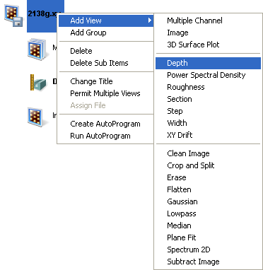
Figure 2: Select Depth from the Workspace

Right-click on a thumbnail in the Multiple Channel window and select Depth.

Select Analysis > Depthfrom the menu bar.

Click the Depth icon in the toolbar.

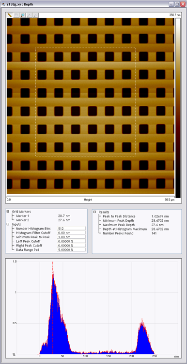
Figure 3: Depth Analysis Menu & Window

Using the mouse, left-click and drag a box on the area of the image to analyze. The Histogram displays the depth correlation on this specified area.

NOTE: If no box is drawn, by default, the entire image is selected.

Adjust the Minimum Peak to Peak to exclude non relevant depths.
Adjust the Histogram Filter Cutoff parameter to filter noise in the histogram as desired.
Note the results.

NOTE: To save or print the data, run the analysis in an Auto Program

Depth Interface

The Depth interface includes a captured image, Grid Markers, Input parameters, Results parameters and a correlation Histogram as shown in Figure 4.

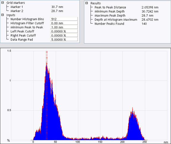
Figure 4: The Depth Interface

Parameter	Description
Number of Histogram Bins	The number of data points which result from the filtering calculation. Note: Having more histogram bins than pixels is unnecessary.
Histogram Filter Cutoff	Lowpass filter which smoothes out the data by removing wavelength components below the cutoff. Use to reduce noise in the Correlation histogram.
Minimum Peak To Peak	Sets the minimum distance between the maximum peak and the second peak marked by a cursor. The second peak is the next largest peak to meet this distance criteria.
Left Peak Cutoff	The left (smaller in depth value) of the two peaks chosen by the cursors. Value used to define how much of the left peak is included when calculating the centroid. Note: At 0%, only the maximum point on the curve is included. At 25%, only the maximum 25% of the peak is included in the calculation of the centroid.
Right Peak Cutoff	The right (larger in depth value) of the two peaks marked by the cursors. Value used to define how much of the right peak is included when calculating the centroid. Note: At 0%, only the maximum point on the curve is included. At 25%, only the maximum 25% of the peak is included in the calculation of the centroid.
Data Range Pad	Creates a buffer region at either end of the histogram.

Table 1: Depth Input Parameters

Parameter	Description
Peak to Peak Distance	Depth between the two data peak centroids as selected using the line cursors.
Minimum Peak Depth	The depth of the deeper of the two features.
Maximum Peak Depth	The depth of the shallower of the two features.
Depth at Histogram Maximum	Depth at the maximum peak on the histogram.
Number of Peaks Found	Total number of peaks included within the data histogram.

Table 2: Depth Results Parameters

Using the Grid Display

Right-clicking on the grid will bring up the Grid Parameters menu.

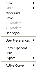
Figure 5: Grid Parameters Menu

Right-clicking on the grid will bring up the Grid Parameters menu (see Figure 5) and allow you to make the following changes:

Parameter	Description
Color	Allows operator to change the color of the: Curve (data) Text Background Grid Minor Grid Markers
Filter	Typically used for a Profiler Scan Type - Select None, Mean (defualt), Maximum, or minimum Points - Select 4k, 8k (default), 16k, or 32k
Minor Grid	Allows user to auto scale, set a curve mean, or set their own data range
Scale	For each curve, the operator can choose a connect, fill down, or point line.
Line Style	Total number of peaks included within the data histogram.
User Preferences	Restore—Reverts to initial software settings Save—Saves all changes operator has made during this session. This becomes the new default settings.
Copy Clipboard	Copies the grid image to the Microsoft Clipboard
Print	Prints out the current screen view to a printer
Export	Exports data in bitmap, JPEG or XZ data format
Active Curve	Determines which curve you are analyzing

Table 3: Plot Appearance Parameters

www.bruker.com	Bruker Corporation
www.brukerafmprobes.com	112 Robin Hill Rd.
nanoscaleworld.bruker-axs.com/nanoscaleworld/	Santa Barbara, CA 93117

	Customer Support: (800) 873-9750
	Copyright 2010, 2011. All Rights Reserved.