Width

|
To analyze the width of features you have numerous choices which measure the height difference between two dominant features that occur at distinct heights. Width was primarily designed for automatically comparing feature widths at two similar sample sites (e.g., when analyzing etch depths on large numbers of identical silicon wafers).
|
The Width command is designed to automatically measure width between features distinguished by height, such as trenches and raised features.
The Width command is best applied when comparing similar features on similar sites. Width measurement on dissimilar sites is better performed using the Section command.
Width Theory
The Width algorithm utilizes many of the same functions found in Depth analysis by accumulating height data within a specified area, applying a Gaussian low-pass filter to the data (to remove noise), then rapidly obtaining height comparisons between two dominant features. For example, [1] the depth of a single feature and its surroundings; or, [2] depth differences between two or more dominant features. Although this method of width measurement does not substitute for direct, cross-sectioning of the sample, it does afford a means for comparing feature widths between two or more similar sites in a consistent, statistical manner.
The Width window includes a top view image and a histogram; depth data is displayed in the results window and in the histogram. The mouse is used to resize and position the box cursor over the area to be analyzed. The histogram displays both the raw and an overlaid, Gaussian-filtered version of the data, distributed proportionally to its occurrence within the defined bounding box.
Histogram
Raw Data
Histograms for depth data are presented on the bottom of the Width window. The histogram peaks correspond to the distribution of depths of analyzed regions of the image (see Figure 1).
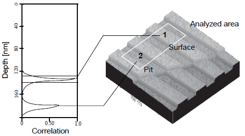
Figure 1: Width Image and Corresponding Histogram
NOTE: Color of cursor, data, and grid may change if user has changed the settings. Right-click on the graph and go to Color if you want to change the default settings.
Correlation Curve
The Correlation Curve is a filtered version of the Raw Data Histogram and is represented by a red line on the Depth Histogram. Filtering is done using the Histogram Filter Cutoff parameter in the Inputs parameter box.The larger the filter cutoff, the more data is filtered into a Gaussian (bellshaped) curve. Large filter cutoffs average so much of the data curve that peaks corresponding to specific features are unrecognizable. On the other hand, if the filter cutoff is too small, the filtered curve may appear noisy.
The Correlation Curve portion of the histogram presents a lowpass, Gaussian-filtered version of the raw data. The low-pass Gaussian filter removes noise from the data curve and averages the curve’s profile. Peaks which are visible in the curve correspond to features in the image at differing widths.
Peaks do not show on the correlation curve as discrete, isolated spikes; instead, peaks are contiguous with lower and higher regions of the sample, and with other peaks. This reflects the reality that features do not all start and end at discrete depths.
When using the Widthview for analysis, each peak on the filtered histogram is measured from its statistical centroid (i.e., its statistical center of mass).
Width Procedure
| |
- Select an image file from the file Browse window at the right of the main window. Double click the thumbnail image to select and open the image.
- You can open the Width view, shown in Figure 3, using one of the following methods:
- Right-click on the image name in the Workspace and select Add View > Width from the popup menu. See Figure 2.
|
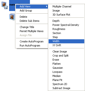
Figure 2: Select Width from the workspace
| |
Or
- Right-click on a thumbnail in the Multiple Channel window and select Width.
Or
- Select Analysis > Width from the menu bar.
Or
|
|
|
- Click the Width icon in the NanoScope toolbar.
|
| |
- The Width view, shown in Figure 3, appears showing results for the entire image.
|
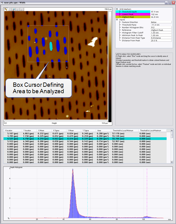
Figure 3: The Width interface
Width Interface
The Width interface includes a captured image, Input parameters and Grid Markerdisplay, Results table, Guidelines and a Depth Histogram with grid markers, shown in Figure 4.
| |
- Using the mouse, left click and drag a box around a particular section of the image. The analysis automatically adjusts the results.
NOTE: If no box is drawn, by default, the entire image is selected.
- Adjust the Minimum Peak to Peak to exclude non relevant depths.
- Adjust the Histogram Filter Cutoff parameter to filter noise in the histogram as desired.
- Adjust the Threshold Depth cursor, shown in Figure 4, along the histogram to set the level of the cutoff plane. The features above or below (depending on Feature Direction) this plane are a single shade in the selected area.
- Right-click on the image in a region outside the box and click Select Feature.
- Click on various regions inside of the box. Statistics in the table will be generated for each distinct (as defined by the Input parameters) feature.
- To save or print the data, either copy, by right-clicking on the results table, and paste the text and export the graphic or XZ data.
|
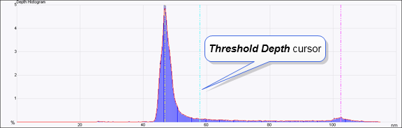
Figure 4: The Depth histogram
Width Parameters
The depth input parameters below define the slider cursor placement for determining the exact depth of a feature.
| Parameter |
Description |
|
Feature Direction
|
Select Above or Below to indicate if features above or below the reference
plane are to be analyzed. |
|
Threshold Plane
|
The Z height which is used as a minimum for the higher peak. This can be
adjusted by moving the cyan Threshold Depth cursor in the depth histogram. |
|
Number of Histogram Bins
|
The number of data points, ranging from 4 to 512, which result from the filtering
calculation. |
|
Reference
|
You may specify a reference point for the cursor. This feature is useful for
repeated, identical measurements on similar samples. After moving the cursor
to a specific point on the correlation histogram, that point is saved as a
distance from whatever reference peak you choose. These reference peaks
include: Highest Peak, Lowest Peak. |
|
Histogram Filter Cutoff
|
Lowpass filter which smoothes out the data by removing wavelength components
below the cutoff. Use to reduce noise in the Correlation histogram. |
|
Minimum Peak To Peak
|
Sets the minimum distance between the maximum peak and the second
peak marked by a cursor. The second peak is the next largest peak to meet
this distance criteria. |
|
Distance From Peak
|
% Distance, Absolute Distance |
|
Distance From Peak
|
Cursor distance from the Reference peak |
Table 1: Width Parameters
Three user-adjustable markers are placed on the depth histogram:
| Parameter |
Description |
|
Threshold Depth
|
Cyan. Distance from peak and distance from peak type. |
|
Lowest Peak
|
Magenta. The right (larger in depth value) of the two peaks marked by the
cursors. |
|
Highest Peak
|
Gold. The left (smaller in depth value) of the two peaks chosen by the cursors.
You can adjust min and max peaks by adjusting the Minimum
Peak To Peak. |
Table 2: Grid Markers
| Parameter |
Description |
|
X location
|
X location |
|
Y location
|
Y location |
|
X mean
|
The average of the highlighted X values within the enclosed area. |
|
X sigma
|
The standard deviation of the measured X values. |
|
Y mean
|
The average of the highlighted Y values within the enclosed area. |
|
Y sigma
|
The standard deviation of the measured Y values. |
|
Area
|
The area below the threshold in the selected region. |
|
Threshold to Local Minimum
|
The distance from the Threshold Plane to a local minimum. |
|
Threshold to Local Maximum
|
The distance from the Threshold Plane to a local maximum. |
Table 3: Results Parameters
| www.bruker.com
|
Bruker Corporation |
| www.brukerafmprobes.com
|
112 Robin Hill Rd. |
| nanoscaleworld.bruker-axs.com/nanoscaleworld/
|
Santa Barbara, CA 93117 |
| |
|
| |
Customer Support: (800) 873-9750 |
| |
Copyright 2010, 2011. All Rights Reserved. |
Open topic with navigation