You are here: NanoScope Software User Guide > Offline Commands > Modify Commands > Flatten

Flatten

	The Flatten command eliminates unwanted features from scan lines (e.g., noise, bow and tilt). It uses all unmasked portions of scan lines to calculate individual least-square fit polynomials for each line.
	Flatten is useful prior to image analysis commands (e.g., Depth, Roughness, Section, etc.) where the image displays a tilt, bow or low frequency noise, which appear as horizontal shifts or stripes in the image.

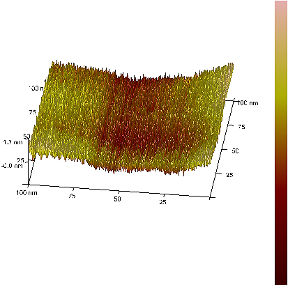
Figure 1: Image with Bow

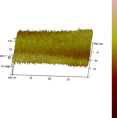
Figure 2: Image with Bow Removed

Flatten Theory

The Flatten command is a filter that modifies the data to delete low frequency noise and remove tilt from an image. Each line is fit individually to center data (0th order) and remove tilt (1st order), or 2nd or 3rd order bow. A best fit polynomial of the specified order is calculated from each data line and then subtracted out. In some cases, the stopband (box cursor to exclude features) can be used to remove regions of the image from the data set used for the polynomial fits. Click on the image to start drawing a stopband box. Right-click on a box to delete it or change its color.

Flatten Polynomials

The polynomial equations calculate the offset and slope, and higher order bow of each line for the data as per the table below.

Order	Polynomial	Explanation
0	z = a	Centers data along each line.
1	z = a + bx	Centers data and removes tilt on each line (i.e. calculates and removes offset (a) and slope (b).
2	z = a + bx + cx ²	Centers data and removes the tilt and bow in each scan line, by calculating a second order, least-squares fit for the selected segment then subtracting it from the scan line.
3	z = a + bx + cx² + dx³	Centers data and removes the tilt and bow in each scan line, by calculating a third order, least -squares fit for the selected segment then subtracting it from the scan line.

Table 1: Flatten Polynomials

Flatten Procedure

	For an image that contains a number of noisy scan lines, use the Flatten command to correct the problem.
	Select an image file from the file browsing window at the right of the main window. Double click the thumbnail image to select and open the image.
	You can open the Flatten view, shown in , using one of the following methods: Right-click on the image name in the Workspace and select Add View > Flatten from the popup menu. See Figure 3.

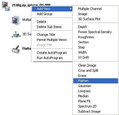
Figure 3: Select Flatten from the Workspace.

Right-click on a thumbnail in the Multiple Channel window and select Flatten.

Select Modify > Flatten from the menu bar.

Click the Flatten icon in the toolbar.

Set the Flatten Order to 0th. This removes the scan line misalignment.

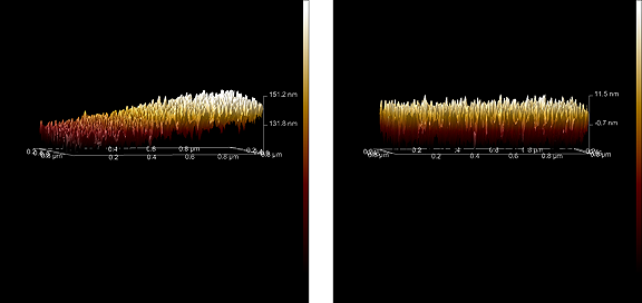
Figure 4: Image of tip check sample before (left) and after (right) 0th order Flatten operation

To see the variety of effects using the Flatten command, enter different Flatten Order values. Each new change may be undone by clicking on the Reload button.

Flatten Interface

A series of parameters appear in the Flatten view, allowing the order of the Flatten polynomial to be selected and display parameters to be adjusted.

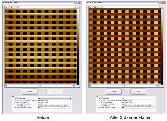
Figure 5: Flatten view—single monitor

Input Parameters

Parameter	Description
Flatten Order	Flatten Order selects the order of the polynomial calculated and subtracted from each scan line. Settings: 0th—Removes the Z offset between scan lines by subtracting the average Z value for the unmasked segment from every point in the scan line. 1th—Removes the Z offset between scan lines, and the tilt in each scan line, by calculating a first order, least-squares fit for the unmasked segment then subtracting it from the scan line. 2nd—Removes the Z offset between scan lines, and the tilt and bow in each scan line, by calculating a second order, least-squares fit for the unmasked segment then subtracting it from the scan line. 3rd—Removes the Z offset between scan lines, and the tilt and bow in each scan line, by calculating a third order, least-squares fit for the unmasked segment then subtracting it from the scan line.
Flatten Z Thresholding Direction	Specifies the range of data to be used for the polynomial calculation based on the distribution of the data in Z: Range or Settings: Use Z >= —Uses the data whose Z values are greater than or equal to the value specified by the Z thresholding %. Use Z <—Uses the data whose Z values are less than the value specified by the Z thresholding %. No thresholding—Disables all thresholding parameters.
Flatten Threshold for	Applies the Thresholding values for the whole image or each line independently. Range or Settings: The whole image Each line
Flatten Z Threshold %	Defines a Z value as a percentage of the entire Z range in the image (or data set) relative to the lowest data point.
Output File Name	Specifies the name of the file to be created. Leave blank for immediate view/use without saving the altered image file.
Write File Upon Execute	Writes the output file when the Execute button is clicked.

Table 2: Flatten Range, Settings and Buttons

Parameter	Description
Execute	Initiates the Flatten command, based on the order selected..
Reload	Restores the image to its original form by reloading the original file.

Table 3: Buttons on the Flatten Panel

www.bruker.com	Bruker Corporation
www.brukerafmprobes.com	112 Robin Hill Rd.
nanoscaleworld.bruker-axs.com/nanoscaleworld/	Santa Barbara, CA 93117

	Customer Support: (800) 873-9750
	Copyright 2010, 2011. All Rights Reserved.