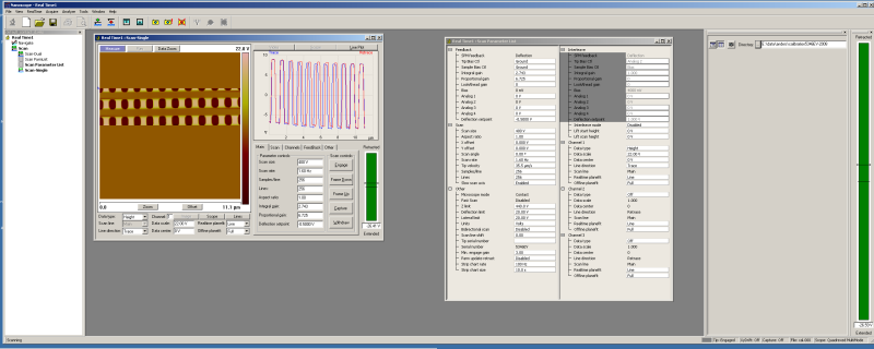
Overview of desktop in ver. 6.
Therefore the scanner has to be calibrated so that the software "knows" how much the scanner is moved for a certain applied voltage. This is shortly described in this web-page for software version 6.
You must also refer to the chapter about calibration in the printed manual for the Nanoscope system, Veeco, formerly Digital Instruments.
Here is an overview of the desktop for the version 6 of the SPM controlling software. From left to right:
This method MUST be used for calibration.
You will get a prompt to set it if it is not active.
A calibration sample with a known pattern size is used. With the system is currently two scanners:
| Scanner | Serial # | Max. Scan area | Ref. sample |
|---|---|---|---|
| J | 5337EJ | 100 × 100 µm | 10 µm pitch, square grid |
| E | 5346EV | 10 × 10 µm | 1 µm pitch, square grid |
The reference sample is a matrix of squares etched down to 200 nm below surface with a size of roughly half the pitch. Please remember that it is the pitch that is the reference distance, not the size of each square.
The calibration is done in three steps:
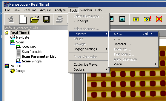
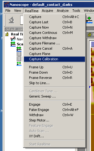
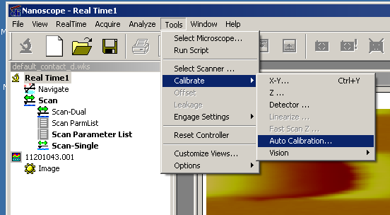
To start the adjustment of linearity and center compression/expansion use drop-down menu Tools —> Calibrate —> X-Y... to start a special scanning window used for these adjustments.
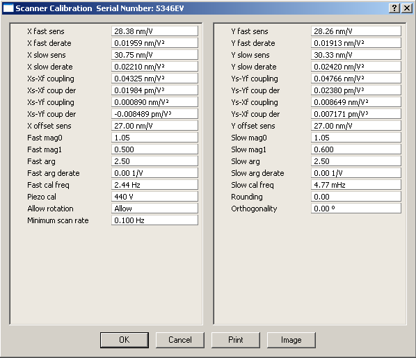
A new window showing all the parameters for the scanner is popped up.
Click button Image, this will extend the window with a live image scan.
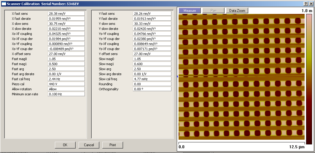
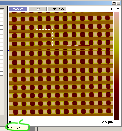
To start measure, click and drag in the image window. A rectangle will be displayed and its x-y size is shown in the lower left corner (marked in green). The size-values should be near the reference values unless the initial calibration done at the factory is seriously wrong.
Size the window by clicking and dragging at the borders of the rectangle. Set the size so that it is equal to 2 × the pitch, i.e. covering two periods of the reference pattern.
Compare the size of the scanned pattern at the first third of the scan with the size at the last third of the scan. All this is described in detail in the calibration chapter in the printed manual. Follow the instructions to adjust linearity and center compression/expansion.
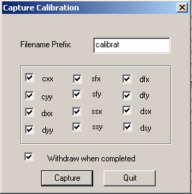
Here is decided which parts of the calibration is to be performed. Usually all variants should be ticked. All images will have a filename according to the prefix with a suffix according to the type of calibration, cxx, cyy etc.
To start click Capture.
During the capture there is a window for adjustments of capture. The four first images are scanned either horizontally or vertically, much like when scanning with Slow Scan Axis = Disabled. Then the user have to adjust so that the scan line is completely across the squares. Here it is a horizontal scan that can be adjusted up or down to scan over the center of a row of reference squares.
The Skip button is to increase the number of image scans that are skipped before the actual capture takes place. The two first images are always skipped in order for the piezos to settle in the scan mode.
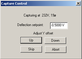
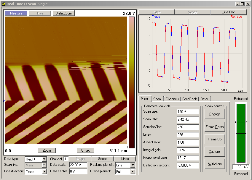
Here is an image being scanned during adjustment, the new image is being scanned from top to bottom, i.e. it is the upper half that is the current image.
During the scanning the offset buttons were clicked to center the scan-line on a row of reference squares. The irregular scan-lines in the upper third of the image are disturbances from the adjustment.
Twelve images are captured, one for each type of parameter to be calibrated. This takes about an hour in total. The four first images needs the user adjustment during scanning, as described above. The rest should not need user attention unless temperature drift makes the Z-piezo go to either fully extended or fully retracted.
The calibration capture can be stopped and continued, only tick in the types of images that are missing. See the Capture Calibration start window.
Select the folder where the calibration images were stored, select the first image, click Open.
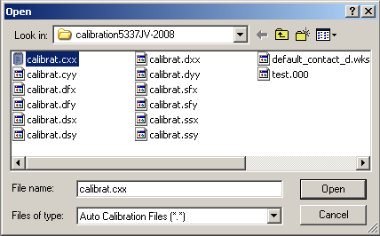
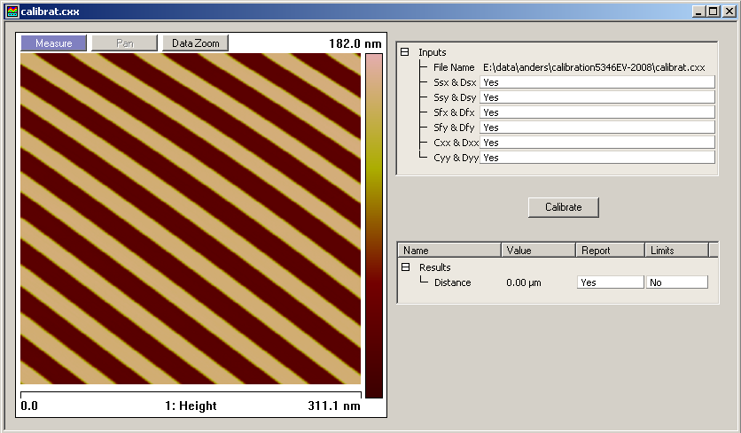
The calibration image called calibrat.cxx
is displayed.
To the right is a list of
parameters to calibrate. In most cases they should all be set to
Yes.
Start the calibration by clicking the Calibrate
button.
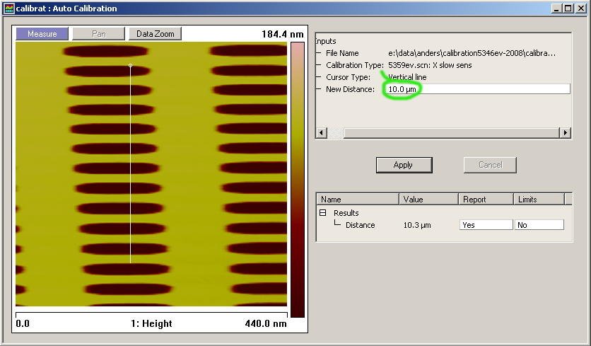
The image belonging to the first parameter to be calibrated, is displayed. You can only draw a vertical line in the image.
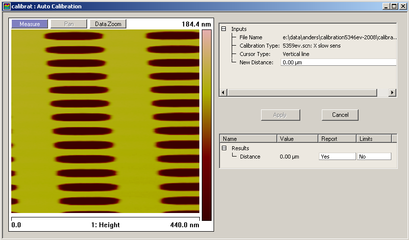
You can only draw vertically, start at a well defined boundary and count
a whole number of periods.
Do not start the line at the very edge of the image, start some 10-20 %
inside the image.
One period is equal to the pitch of the reference
sample.
In this image ten periods are indicated by the vertical line. Please note
that the little info-square is showing completely wrong information.
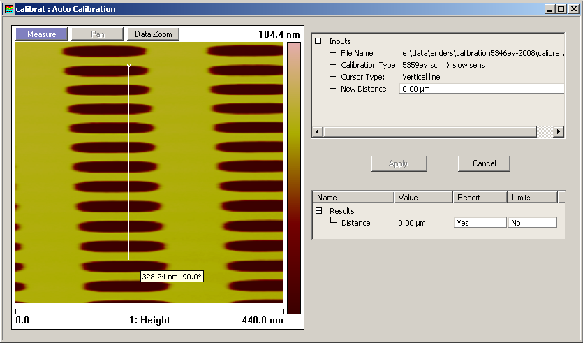
When the mouse button is released the software "guess" the actual
distance, it is displayed in the
New Distance-entry.
It should normally be rather close to the real distance given by the known
reference sample pitch.
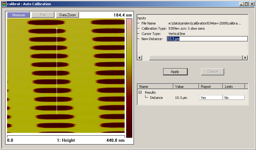
Next the user enters the known distance value as given by the number
of periods spanned by the line,
in this case 10 × 1 µm.
The "E"-scanner is used in this example, it requires a reference
sample with a pitch of 1 µm.
Click
Apply-button, the parameters are recalculated
according to the new distance given, and the next calibration image is
displayed.
The next image is displayed, draw vertical line over an integer number of periods, and give the true length value, click Apply.
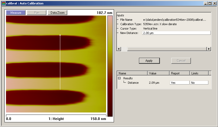
And so on...
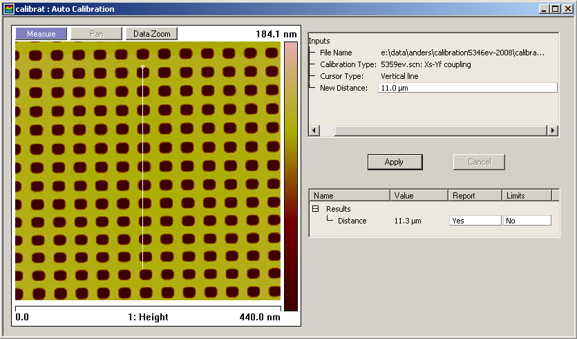
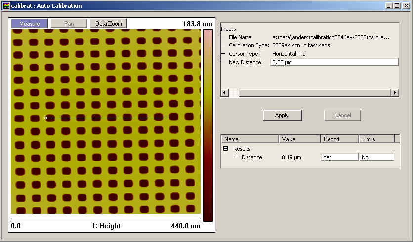
Some image require a horizontal line instead.
When all images have been measured, the pop-up below appears instead
of a new calibration image.
The calibration data has been re-computed and the calibration file
is re-written.
In order to use the new calibration parameters you must re-load the workspace.