Section

The Section command displays a top view image, upon which up to three reference lines may be drawn. The cross-sectional profiles and fast Fourier transform (FFT) of the data along the reference lines are shown in separate windows. Roughness measurements are made of the surface along the reference lines you define.

Section is probably the most commonly used Analysis command; it is also one of the easiest commands to use. To obtain consistently accurate results, ensure your image data is corrected for tilt, noise, etc. before analyzing with Section.

Sectioning of Surfaces

Samples are sectioned to learn about their surface profiles. The Section command does not reveal what is below the surface—only the profile of the surface itself. When sectioning samples, it is important to ascertain surface topology before applying the Section analysis. Depending upon the topology and orientation of the sample, the results of Section analysis may vary tremendously.

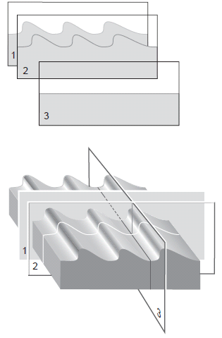
Figure 1: Examples of Section Analysis

The sample surface above (a diffraction grating) is sectioned along three axes. Sections 1 and 2 are made perpendicular to the grating’s rules, revealing their blaze and spacing. (Sections 1 and 2 may be compared simultaneously using two fixed cursor lines, or checked individually with a moving cursor.) Section 3 is made parallel to the rules, and reveals a much flatter profile because of its orientation.

The Section command produces a profile of the surface, then presents it in the Cross Section Plot.

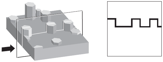
Figure 2: Cross Section Plot Profile

Generally, Section analysis proves most useful for making direct depth measurements of surface features. By selecting the type of cursor (Rotating Line, Rotating Box, or Horizontal Line), and its orientation to features, you may obtain:

• Vertical distance (depth), horizontal distance and angle between two or more points.
• Roughness along section line: RMS, R_a, R_max, R_z.
• FFT spectrum along section line.

Features are discussed below. Refer to Roughness for additional information regarding roughness calculations.

Section Procedure

To perform Section analysis:

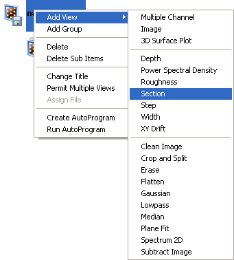
Figure 3: Select Section from the workspace

	Or Right-click on a thumbnail in the Multiple Channel window and select Section. Or Select Analysis > Section from the menu bar. Or
	Click the Section icon in the NanoScope toolbar.
	The Section view, shown in Figure 4, appears showing results for the entire image.

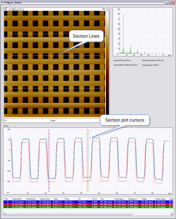
Figure 4: The Section view

To remove any tilt which might be present, select Modify > Plane Fit or click the Plane Fit icon on the NanoScope toolbar. Set the Plane Fit Order parameter in the panel to 1st, then click the Execute button. The image is fitted to a plane (“leveled”) by fitting each scan line to a first-order equation, then fitting each scan line to others in the image. At this point, the image has not been appreciably altered, it has only been reoriented slightly.

In Section Analysis, to make a single-line section of the image, use the mouse to draw a line through the image, as in Figure 5, and note the results. Move the grid cursors along the section to make measurements. Additional lines may be drawn on the image in the same fashion as the first. Up to three Section lines may be drawn on the image at any one time. A Section line may be moved on the image by clicking and dragging the center of the line. A Section line may be deleted by right clicking and selecting "delete."

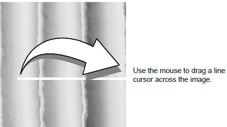
Figure 5: Mouse Drawing Line

Section Interface

When a line is drawn on the image, the cross-sectional profile is displayed, and the FFT spectrum along the line is also displayed (see Figure 4). More detail about the FFT algorithm used may be found at http://www.fftw.org.

The markers may be positioned in the profile and FFT spectrum. The results window at the bottom of the display lists roughness information based on the position of the presently selected reference markers. Each marker pair is color coordinated with the data in the results window.

Grid Markers:

A pair of markers in the section grid and a single marker in the spectrum grid will automatically be drawn. Place the mouse cursor on the desired marker and left-click to move.

Table 1: Grid Markers

Section Results

The Results window at the bottom of the display lists roughness information based on the position of the presently selected reference markers. Each marker pair is color coordinated with the data in the results window. Data between the two markers will be displayed in the results window at the bottom of the display screen in blue.

The results columns may be customized to display only information you are interested in by right clicking on the results table.

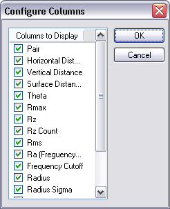
Figure 6: Configure Columns Window - Right-click on Results Table to access

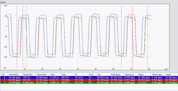
Figure 7: Section results

Result	Description
Horizontal Distance	The measured horizontal distance between the two cursors.
Vertical Distance	The measured vertical distance between the two cursors.
Surface Distance	The distance measured along the surface between the two cursors, including change in translation as well as distance traveled over topography.
Angle	Angle of the imaginary line drawn from the first cursor intercept to the second cursor intercept.
Rmax (Maximum Height)	Difference in height between the highest and lowest points on the cross-sectional profile relative to the center line (not the roughness curve) over the length of the profile, L.
Rz (Ten-Point Mean Roughness)	Average difference in height between the five highest peaks and five lowest valleys relative to the center line over the length of the profile, L. In cases where five pairs of peaks and valleys do not exist, this is based on fewer points.
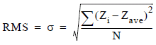
Rms (Standard Deviation)	Standard deviation of the Z values between the reference markers, calculated as: where Zi is the current Z value, Zave is the average of the Z values between the reference markers, and N is the number of points between the reference markers.
Rz Count	The number of peaks used for the Rz computation.
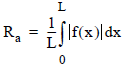
Ra (Mean Roughness)	Mean value of the roughness curve relative to the center line, calculated as: where L is the length of the roughness curve and f(x) is the roughness curve relative to the center line.
Frequency Cutoff (um)	Frequency Cutoff measured in terms of a percentage of the root mean square. Changing the cursor on the FFT changes lc, the cutoff length of the high-pass filter applied to the data. The filter is applied before the roughness data is calculated; therefore, the position of the cutoff affects the calculated roughness values.
Radius	Radius of circle fitted to the data between the cursors.
Radius Sigma	Mean square error of radius calculation.
Length	Length of the roughness curve.
Spectral Period	Spectral period at the cursor position.
Spectral Frequency	Spectral frequency at the cursor position.
Spectral RMS Amplitude	Amplitude at the cursor position.

Table 2: Section Results Columns

Open topic with navigation