Tip Qualification

Tip Qualification refers to estimating tip shape from appropriate characterizer samples and rating tips as good, worn, bad, suspect, or no tip. The Tip Qualification function incorporates the two separate capabilities: Tip Estimation and Tip Qualification.

Tip Estimation

Tip Estimation generates a model of the tip based on an image of a standard characterizer sample. A characterizer refers to a sample whose surface is well suited to deducing tip condition when imaged using an SPM probe.

In Tip Estimation, local peaks in a topographic image are successively analyzed, refining a 3-dimensional tip model. At each peak, the slope away from the peak in all directions is measured, determining the minimum tip sharpness (no data in the image can have a slope steeper than the slope of the tip). As this process is repeated for each local peak, any steeper slope than was found from all previously analyzed peaks causes the tip model to update to a new, sharper tip estimate.

Tip Qualification

Tip Qualification uses the tip estimate to determine whether the tip is acceptable for use. This feature can be used to check tips periodically for signs of wear, and to exchange unacceptably worn tips. By using tip qualification to enforce tip acceptance criteria, metrological values can be compared from image to image, ensuring consistent, long-term comparability of samples.

Theoretical Foundation for Tip Qualification

It is not useful to qualify a probe tip that is poorly matched to the sample to be imaged. Specifically, a tip cannot resolve the linear and angular aspects of any sample feature sharper than the tip itself. (However, even a blunt tip can resolve height accurately on a surface with shallow slopes.) Therefore, select a tip sharp enough to resolve the features of interest.

Tip Artifacts 

Atomic Force Microscope (AFM) images depend on the shape of the tip used to probe the sample. Tip artifacts refer to either the occurrence of features or the absence of features in an image that are not in the sample, but due to the tip used as compared (hypothetically) with an ideal tip of near-zero tip radius. In the simplest case, the finite size of the AFM tip does not allow it to probe narrow, deep fissures in a sample where the tip radius is greater than the radius of the recess.

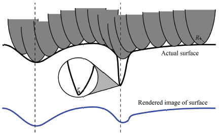
Figure 1: Tip Artifact Depiction

Also, sharp sample features scanned with a dull tip are broadened in AFM images. Consequently, image measurements such as surface roughness and surface area depend on probe tip shape. An image generated with a sharp tip shows greater roughness and larger surface area than an image produced with a dull tip.

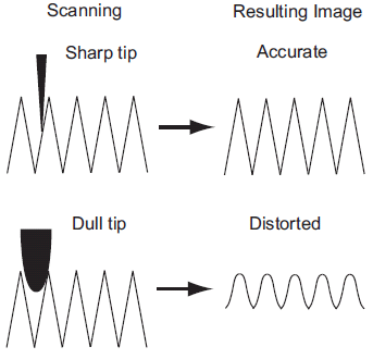
Figure 2: Effects of Tip Sharpness

Sample Dependence of Tip Qualification

The model generated by tip estimation is not, in general, the actual shape of the tip. Because the tip model is constructed by analyzing the shapes of peaks in the image data, the accuracy of the model is limited by the sharpness of features on the characterizer.

Characterizer samples that provide the most accurate estimate of tip size and shape are those with many fine protrusions, since they typically have very sharp features. Even these samples are not perfect, and only a surface with infinitely sharp features can produce an perfectly accurate model of the tip:

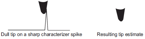
Figure 3: Characterizer - Dull Tip on Sharp Characterizer

A surface having only large rounded features provide the least useful estimate of tip shape:

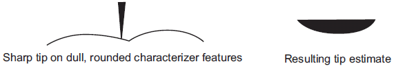
Figure 4: Sharp Tip on Rounded Characterizer

Similar feature size of the characterizer and tip will yield a combined geometry for the tip shape:

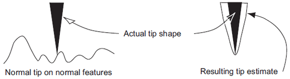
Figure 5: Typical Characterizer

Despite the dependence on characterizer characteristics, Tip Estimation and Tip Qualification can often provide a reliable method of tracking tip wear and ensuring that probes are changed when they become dull. For example, when making repeated measurements on suitable rough samples, Tip Estimation can provide very reproducible estimates of tip size and shape, which change in a predictable and consistent fashion as the tip wears.

Tip Quality Thresholds 

Based on thresholds set by the user, Tip Qualification software usually finds the tip status to be Good, Worn, or Bad.

• A tip status of Good indicates that the tip is still sufficiently sharp and that the image data should be acceptable.
• A tip status of Worn indicates that the tip is becoming dull and should be changed, but previous image data taken with this tip should still be acceptable.
• If a Bad status is returned, the tip should be changed and the current image data discarded.
• In cases where imaging errors are suspected, Tip Qualification may assign a status of Suspect or No Tip.

Characterizer Sample Selection

Just as probe selection influences imaging results, characterizer sample selection influences probe tip characterization. An ideal characterizer sample for tip diagnosis has isolated extremely sharp peaks.

Bruker provides a characterizer sample that is recommended for tip evaluation. The polycrystalline titanium roughness sample (part number RS, available at www.brukerafmprobes.com) has jagged features suitable for obtaining an accurate tip model.

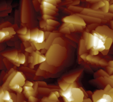
Figure 6: Polycrystalline Titanium Roughness Sample

Operating Principles of Tip Qualification

The result of running Tip Qualification is a display similar to Figure 7.

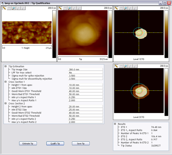
Figure 7: A Typical Tip Qualification Window

The top-left frame is the image analyzed to evaluate the tip. The top-middle frame, labeled Tip, is a top view image of the software model of the tip (looking into its apex).

Once a tip model has been generated, Tip Estimation extracts an estimate of the tip geometry in cross-sections at two different distances from the tip apex, as seen in Figure 8.

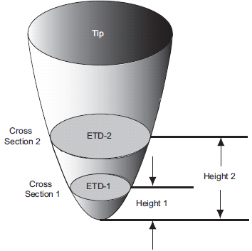
Figure 8: Tip Estimation Cross-Sections Depiction

The cross-section diagrams on the right in Figure 7 show the apparent size and shape of the tip at two different distances from its apex (labeled “Level 1 ETD” and “Level 2 ETD.” In the level 1 cross-section, the roughly circular tip diameter is shown in light gray. In the lower-right frame of Figure 7, the level 1 cross-section is shown again in light gray and the level 2 cross-section is shown darker. (The actual colors of the tip cross-sections depend on the color table selected.)

Tip Estimation then provides, at each cross section, two numerical measures of tip size and shape: effective tip diameter (ETD) and aspect ratio (AR). The effective tip diameter is defined as the diameter of a circle having the same area as the measured tip cross-section (see Figure 9). The ETD is shown below as a circle to the right.

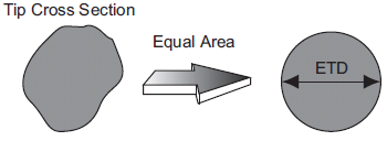
Figure 9: ETD Depiction

Aspect Ratio is defined as the ratio of the maximum vertical (Y) dimension to the maximum horizontal (X) dimension of a tip cross section as seen in Figure 10.

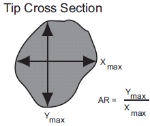
Figure 10: Aspect Ratio Depiction

Control of Tip Qualification Status

Tip Qualification generates a tip status based on the calculated values of ETD, AR and on threshold and limit values selected. There are two ETD thresholds that affect tip status:

• Good/Worn ETD Threshold—If the ETD is smaller than this number, the tip will usually be characterized as Good. The threshold diameters are shown as green circles in the ETD windows.
• Worn/Bad ETD Threshold—If the ETD is smaller than this threshold, but bigger than the Good/Worn ETD Threshold, it is characterized as WORN. If the ETD is larger than this number, it is characterized as BAD. These threshold diameters are shown as red circles in the ETD windows.

There are separate sets of ETD thresholds for the two tip levels (ETD 1 at HEIGHT 1, and ETD 2 at HEIGHT 2). There are also minimum and maximum limits for tip AR at each level. These limits detect when the image data produces a tip model of an oblong shape that is unlikely to accurately represent the tip. Usually an oblong tip model is induced by an imaging artifact, such as a noise streak not removed by discontinuity rejection. The AR limits should not be adjusted.

It takes some experimentation with a particular tip and characterizer sample type to find appropriate values for the various thresholds. The basic idea is to find the maximum ETDs (the diameters of the dullest tips) that provide reliable image data for your samples, then set the Worn/Bad ETD Thresholds based on these diameters. Then set the Good/Worn ETD Thresholds slightly smaller than the Worn/Bad ETD Thresholds.

An additional limit, Min ETD Size, is used to reject Tip Qualification results if the estimated tip is unreasonably small (indicating a tip that is sharper than physically likely). This is usually induced by imaging artifacts, such as noise spikes not removed by spike rejection. In most cases, Min ETD Size can be set at or near the same value as the height from the tip apex for both cross sections. So, if Height 1 = 10 nm, a reasonable value for the Min ETD Size is also 10 nm.

Since the tip estimate is valid only where the tip contacts the characterizer sample, cross section heights should be selected to ensure that the tip makes “frequent” contact with the characterizer sample at those heights. Thus, the cross section heights should be below the sample peak-to-valley values. If the cross section heights are too high for the characterizer sample, the resultant ETD will tend to be very large and multiple apparent peaks will be found at that height.

Tip Qualification Procedure

Scan (contact mode) the characterizer sample. Set the scan size to approximately 2.5um. Characterizer image size is important because, along with Tip Image Size and feature density, it determines how many peaks are used for the tip estimation. To accurately estimate the tip shape, there must be many peaks (greater than 10 is good).

Select the captured image file of the characterizer sample from the file browsing window at the right of the main window. Double click the thumbnail image to select and open the image. You can open the Tip Qualification view, shown in Figure 12 using one of the following methods:  Right-click on the image name in the Workspace and select Add View > Tip Qualification from the popup menu. See Figure 11.

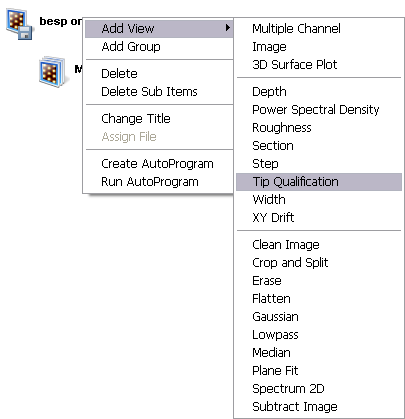
Figure 11: Select Tip Qualification from the workspace

	Or Right-click on a thumbnail in the Multiple Channel window and select Tip Qualification. Or Select Analysis > Tip Qualification from the menu bar. Or
	Click the Tip Qualification icon in the NanoScope toolbar.
	The Tip Qualification window, shown in Figure 12, appears.

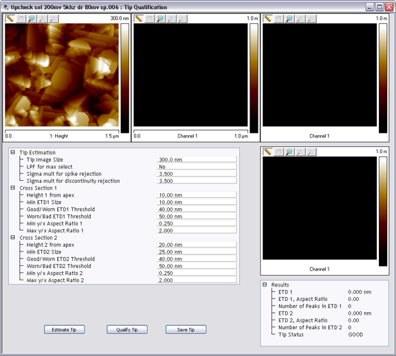
Figure 12: The Tip Qualification window before calculations

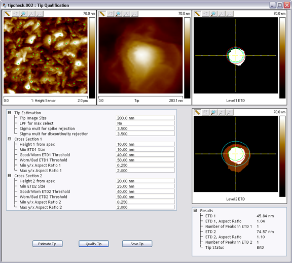
Figure 13: Tip qualification results

If the end radius of the tip is required, click Save Tip and then open the saved file. Click the Section icon to open the file and draw a cursor through the tip center, shown in Figure 14. The radius of a circle fitted to the data between the cursors is displayed in the bottom of the Section window. See Section for more information.

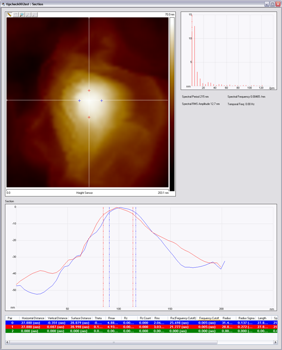
Figure 14: Section of the saved tip

Tip Qualification Interface

Tip Qualification Buttons

Table 1: Tip Qualification buttons

Group	Parameter	Description
Tip Estimation	Tip Image Size	Sets the size of the image displayed in the upper-left corner of the Tip Qualification window. Calculated tip diameters are not expected to exceed Tip Image Size. For example, Tip Image Size = 120 NM will result in a tip image approximately 120 nm square. A reported ETD is the smallest odd integer multiple of the sample data resolution that is greater than or equal to the calculated tip diameter. Tip Image Size also defines in a characterizer image the neighborhood size used to select the topographic maxima points used for Tip Estimation. For example, for Tip Image Size = 120 NM, each selected maximum pixel is the tallest point topographically within an approximately 120 nm square centered on the point. Therefore, a larger Tip Image Size may result in fewer selected maxima. More points provide more tip information, so select Tip Image Size to be as small as possible while also satisfying two other conditions: 1) Tip Image Size should exceed the ETD at as tall a height above the tip apex as is contacted imaging the characterizer sample. Determine this experimentally by varying Tip Image Size and observing the resultant top-middle image in the Tip Qualification window. NOTE: A good starting point for Tip Image Size is the sum of the maximum allowable tip diameter plus the diameter of a typical feature in the characterizer. 2) If and when “double tip” peaks appear in the image due to tip wear, their apexes should be no farther apart than one-half Tip Image Size. This ensures that multiple peaks from a “double tip” feature are not treated as separate features from the same peak (which would produce erroneous results and no longer guarantee an outside tip envelope). NOTE: Characterizer image size and feature density also affect the number of selected maxima.
	LPF for max select	Determines whether a lowpass filter is applied to the data before identifying selected points. The filtered data is only used for point selection, not for the actual tip calculation. This filter has the effect of reducing noise sensitivity. It is recommended that the filter be turned on (Yes).
	Sigma Mult for spike rejection	Sets a threshold for rejection of isolated upwards-oriented noise spikes. At each point (x,y) in an image, a difference Δ(x,y) is calculated between the pixel value at that point and the average value of the surrounding eight pixels. The average, μ, and standard deviation, σ, of all positive Δ(x,y)s in the image are then calculated. The normal (Gaussian) distribution with average value, μ, and standard deviation, σ, is then used to represent the actual distribution of positive Δ(x,y) values. If the value of Sigma mult for spike rejection is M, then points (x,y) whose Δ(x,y) value differs from μ by more than M*σ are rejected as local maxima in Tip Estimation. The algorithm rejects as noise any unusually large pixel values as compared to the neighboring pixels. Because most pixel values are close to the average value of their neighbors, the Δ(x,y) distribution is skewed toward zero. If Sigma mult for spike rejection = 0, noise spike rejection is not performed. If the parameter value is > 0, noise spike rejection is performed.
	Sigma Mult for discontinuity rejection	Similar to Sigma mult for spike rejection (above), this parameter sets a threshold for rejection of entire rows of data where a discontinuity is detected, such as when the tip “trips” over a feature. If Sigma mult for discontinuity rejection = 0, discontinuity rejection is not performed. If the parameter is > 0, discontinuity rejection is performed as follows: for each row y, the average absolute value δy of the differences between each point and its immediate neighbor on the next line is calculated. The average μ and standard deviation σ of all such average differences δy is computed. 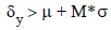Rows are rejected for a discontinuity where δy meets the following criterion: where M is Sigma mult for discontinuity rejection. Points which fall within a Tip Image Size neighborhood centered on a discontinuity row are disqualified from contributing to Tip Estimation. Discontinuity rows are displayed as red horizontal lines on the image display.
Cross Section 1		Tips are cross-sectionally analyzed at two separate heights above the apex to determine tip status. These heights correspond to Cross Section 1 and Cross Section 2. Parameters are appended with either a “1” or a “2,” depending on which cross section they describe (e.g., Height 1 and Height 2, respectively). NOTE: If cross-sectional analysis is desired at only one height, set Height 1 to 0.00 nm, and set Height 2 to the desired value.
	Height 1 from Apex	Distance from the tip apex at which the cross section is defined.
	Min ETD1 Size	Minimum credible ETD at Cross Section 1. If the calculated ETD is smaller than Min ETD Size, then Tip Status = Suspect.
	Good/Worn ETD1 Threshold	Maximum ETD1 assigned Tip Status = Good (assuming that no other conditions such as an unacceptable aspect ratio or the presence of discontinuities result in a Suspect Tip Status).
	Word/Bad ETD1 Threshold	Maximum ETD1 assigned Tip Status = Worn. If ETD1 is greater than Worn/Bad ETD1 Threshold then Tip Status = Bad.
	Min y/x Aspect Ratio 1	Maximum AR1 assigned Tip Status = Suspect if ETD1 is less than Worn/Bad ETD1 Threshold.
	Max y/x Aspect Ratio 1	Minimum AR1 signed Tip Status = Suspect if ETD1 is less than Worn/Bad ETD1 Threshold.
Cross Section 2	Height 2 from Apex	Distance from the tip apex at which the cross section is defined.
	Min ETD2 Size	Minimum credible ETD at Cross Section 2. If the calculated ETD is smaller than Min ETD Size, then Tip Status = Suspect.
	Good/Worn ETD2 Threshold	Maximum ETD2 assigned Tip Status = Good (assuming that no other conditions such as an unacceptable aspect ratio or the presence of discontinuities result in a Suspect Tip Status).
	Word/Bad ETD2 Threshold	Maximum ETD2 assigned Tip Status = Worn. If ETD2 is greater than Worn/Bad ETD2 Threshold then Tip Status = Bad.
	Min y/x Aspect Ratio 2	Maximum AR2 assigned Tip Status = Suspect if ETD2 is less than Worn/Bad ETD2 Threshold.
	Max y/x Aspect Ratio 2	Minimum AR2 signed Tip Status = Suspect if ETD2 is less than Worn/Bad ETD2 Threshold.

Table 2: Tip Estimation Panel Parameters

Table 3: Tip Status Results - Evaluated in the Following Order

Open topic with navigation