|
|
The Gaussian filter applies either a Lowpass or a Highpass digital filter to an image along either the Horizontal or the Vertical axis. |
The Lowpass Gaussian Filter eliminates high frequency (sharp) features oriented along either the X or Y axis of the scan. The practical effect upon the image is a loss of detail or "blurring" effect.
The Gaussian filter can average features running parallel to an image’s Y scan axis while leaving features relatively unchanged along the X axis, or vice versa. This is a similar capability to the Spectrum 2D function, although applied to only the X or Y axis.
Consider the scan of the grating shown in Figure 1, with prominent features oriented along the X axis.
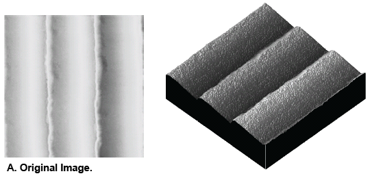
Figure 1: Grating with Prominent X-Axis Features
Applying a Lowpass Gaussian Filter along the Vertical (Y) axis results in elimination of noise in the image.
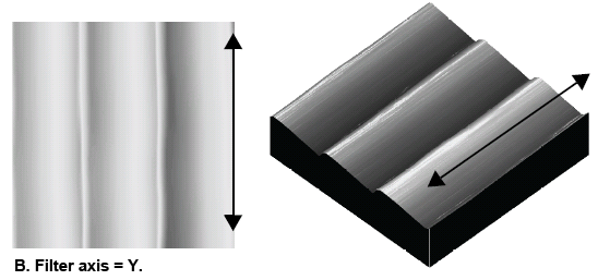
Figure 2: Noise Removed by Applying Lowpass Gaussian Filter to Y Axis
Applying the Lowpass Gaussian Filter to the Horiztonal (X) axis destroys the ruling features in the image by averaging across their profile.
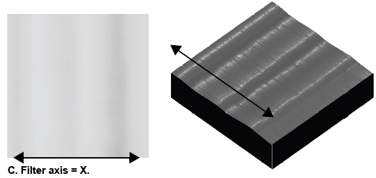
Figure 3: Lowpass Gaussian Filter Applied to Horizontal X Axis
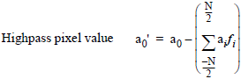
The Highpass Gaussian Filter eliminates low frequency (dull) features oriented along either the X or Y axis of the scan. The "DC" (average) value is also eliminated, resulting in an image containing only the transitions from one region to the next. This filter is typically used for edge detection of different regions or grain bounders.
One example of applying a Gaussian Highpass filter is the magnetic domains in a permalloy specimen, as shown below.
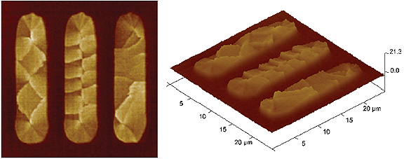
Figure 4: Permalloy Specimen
When the image is filtered using the Horizontal setting, the high frequency features along the X-axis are highlighted.
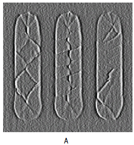
Figure 5: Highpass Gaussian Filter Using Horizontal Setting
When the image is filtered using the Vertical setting, the high frequency features along the Y-axis are highlighted.
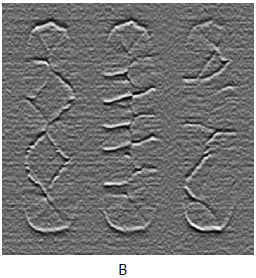
Figure 6: Highpass Gaussian Filter Using Vertical Setting
A composite of the two images shows the domain boundaries clearly. All of the low frequency features have been removed, leaving only the transitions between the grain boundaries.
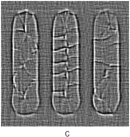
Figure 7: Highpass Gaussian Filter Using Horizontal & Vertical Settings
Gaussian filters utilize a 1 x N matrix, where N is determined by the filter size parameter. In this instance, image data is analyzed in two-dimensional matrices which are shaped to a Gaussian curve where the sigma value (σ) is determined by the filter size parameter.
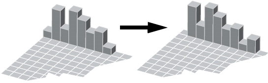
Figure 8: Gaussian Filter Depiction
The general equation used to generate a 1-by-(N+1) Gaussian kernel is:
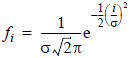
Where i is in units of pixels, and σ is set by the Filter size value. Using this kernel, the filter output is:
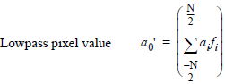
The Filter Size value corresponds to the sigma (σ) value of the Gaussian curve, encompassing approximately 68 percent of the data with the symmetric Gaussian curve centered over the operated-upon pixel.
Larger Filter size values distribute the curve broadly.
During Lowpass filtering, this lends greater weight to values farther away from the pixel and increases the Gaussian filter’s averaging effects upon the image.
During Highpass filtering, this subtracts a decreased average from each pixel, lessening the filter’s impact.

Figure 9: Larger Filter Size
Smaller Filter size values concentrate curve data around the center value.
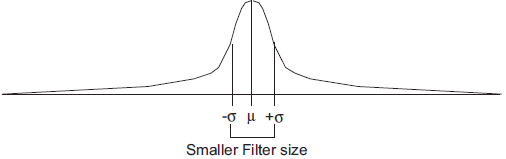
Figure 10: Smaller Filter Size
During Lowpass filtering, this lends less weight to pixels distant from the center, decreasing the Gaussian filter’s ability to average local pixels with distant ones—the filter’s impact is lessened.
During Highpass filtering, the larger and more localized pixel average being subtracted from the operated-upon pixel value yields an enhanced impact upon the image.
Filter size is specified in units of Distance, Spatial Frequency, Time, Temporal Frequency, and #pixels.
|
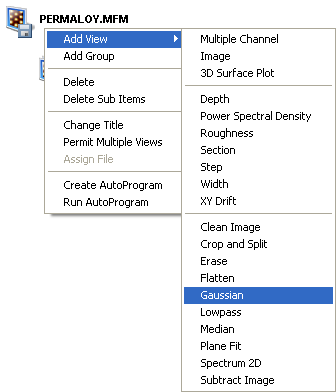
Figure 11: Select Gaussian from the Workspace.
|
Or
Or
Or |
|
|
|
Click the Gaussianicon in the toolbar. |
|
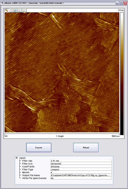
Figure 12: The Gaussian filter panel
|
| Parameter | Description |
|---|---|
|
Filter Size |
Size of the scan line to be operated upon by the Gaussian filter kernel. This value is expressed in the Cutoff Units specified below. Range and Settings:
|
| Filter Axis |
Settings:
|
| Cutoff Units |
Selected units are applied simultaneously to the Filter size. (The #pixels field displays the pixel equivalent of the current Filter Size value.) Range and Settings:
|
| Filter Type |
Range and Settings:
|
| #pixels |
The current Filter size in pixel units. This value may be used to both enter and monitor the Filter size. Range and Settings:
|
| Output File Name | Select the path of the extracted image file. Leave blank for immediate view/use without saving the altered image file |
| Write File Upon Execute | Writes the output file(s) when the Execute button is clicked. |
Table 1: Parameters in the Gaussian Filter Panel
| Button | Action |
|---|---|
|
Execute |
Applies the Gaussian Filter to the currently loaded image. |
|
Reload |
Restores the image to its original form by reloading the original file. |
Table 2: Buttons on the Gaussian Panel
| www.bruker.com | Bruker Corporation |
| www.brukerafmprobes.com | 112 Robin Hill Rd. |
| nanoscaleworld.bruker-axs.com/nanoscaleworld/ | Santa Barbara, CA 93117 |
| Customer Support: (800) 873-9750 | |
| Copyright 2010, 2011. All Rights Reserved. |