
Often, users prefer to Determine Cantilever Spring Constant by Thermal Tune is often preferred over The Added Mass Method (which is more demanding and time-consuming) or Estimation from Cantilever Geometry (which has a large uncertainty factor). The measurement data consists of a time interval of the deflection signal in Contact Mode (i.e., with no driving oscillation applied electronically) at thermal equilibrium, while the cantilever is suspended away from any solid surface. Brownian motion of surrounding (air) molecules impart random impulses to the cantilever during the sampling. The resulting function of time is Fourier transformed to obtain its Power Spectral Density (PSD) in the frequency domain. Integrating the area under the resonant peak in the spectrum yields the power associated with the resonance.
Expressing the dynamics of the cantilever as a harmonic oscillator by the total system energy (the Hamiltonian), the average value of the kinetic and potential energy terms are both
according to the Equipartition Theorem, where:
T = temperature in Kelvin
kB = Boltzmann’s constant, 1.3805 x 10⁻²³joules/Kelvin
In particular, for the potential energy,
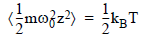
where:
ω0 = (k/m)1/2 is the resonant angular frequency
m = the effective mass
z = the displacement of the free end of the cantilever
The “angle” brackets indicate average value over time.
Simplifying, the temperature and average displacement determine the cantilever spring constant:
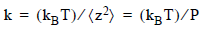
The original displacement time-series is Fourier transformed to segregate other broadband noise contributions from the narrowband thermal noise around resonance. By integrating the area under the resonance in the PSD, while excluding both the noise floor and the “shoulders” to either side of the resonance peak, only the power, P, of the thermal cantilever fluctuations is included. The latter is equal to the mean square of the time-series data. For further discussion of this derivation, refer to Calibration of Atomic-Force Microscope Tips, by Jeffrey L. Hutter and John Bechhoefer, in Review of Scientific Instruments, 64(7): July 1993, page 1868.
The NanoScope V Controller automates the thermal tune calculations. Ten seconds of sampling is sufficient to define the PSD with 25 Hz frequency resolution.
The accuracy of the thermal method of cantilever spring constant determination depends not only on the effective isolation of non-thermal noise contributions to the PSD, but also on the accuracy of the PSD and on its magnitude. The Nyquist Sampling Theorem guarantees Fourier Transform accuracy for frequencies up to one half the sampling rate. The standard NanoScope V Controller samples the deflection signal every 16.5 μs, corresponding to a 64 kHz sampling rate. Therefore, cantilever resonances with contributions from frequencies above 32 kHz can produce distorted PSDs. This particularly constrains using the method for small cantilevers in air. The Thermal Tune technique is mainly applicable to soft cantilevers, particularly in fluids where cantilever resonant frequencies are considerably lower than in air.
Because the magnitude of the PSD is proportional to the average cantilever displacement, higher spring constant (stiffer) cantilevers produce a smaller signal to analyze. For instance, a spring constant of 0.05 N/m produces cantilever displacements of approximately 0.3 nm at room temperature. This is representative of the probes with the smallest spring constants: SiN, NP, NP-STT, DNP, DNP-S (0.01–0.6N/m), and OTR4 (0.02–0.08 N/m) among V-shaped cantilevers, and ESP (0.02-0.1 N/m) among single-beam cantilevers.
| www.bruker.com | Bruker Corporation |
| www.brukerafmprobes.com | 112 Robin Hill Rd. |
| nanoscaleworld.bruker-axs.com/nanoscaleworld/ | Santa Barbara, CA 93117 |
| Customer Support: (800) 873-9750 | |
| Copyright 2010, 2011. All Rights Reserved. |