Responsible: Adrian Iovan, Anders Liljeborg
Icon
Alignment Station Calibration
restricted access
Icon Optics Calibration restricted access
Nanoscope offline software restricted access
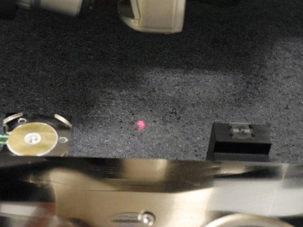
To align the laser on the cantilever, use the two knobs at the top
of the scan head. Observe the laser spot on the stage base.
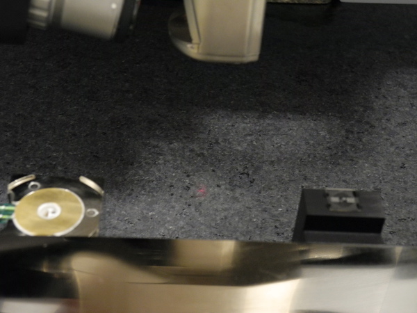
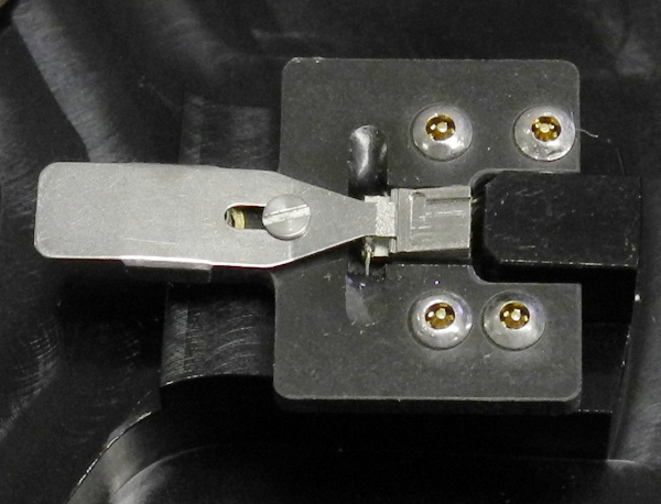
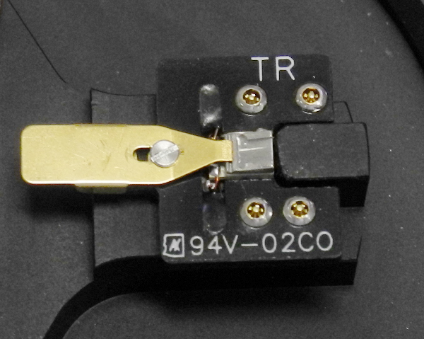
| Here the laser spot is maximally occluded by the cantilever. At the same time the sum signal on the quad detector should be maximum. To see the sum signal of course requires that you already have loaded an experiment in the software, see below. |
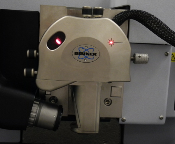
| In the left oval window on the scan-head can now be seen a red elliptical dot, indicating a good reflection of the laser from the back of the cantilever. |
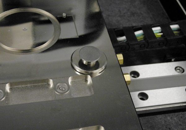
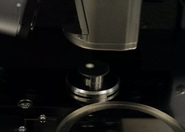
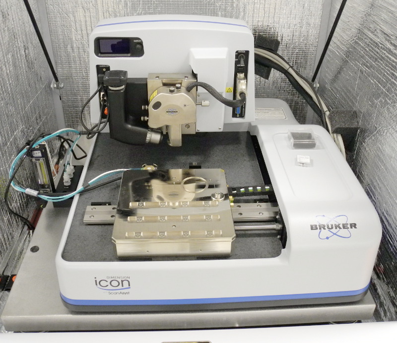
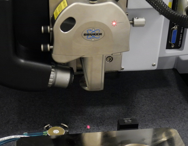
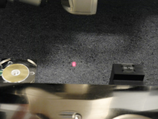
| The scan head is above the steel puck where normally the sample would be mounted. The white small circle is the illumination for the camera. In the center there is a small red dot from the laser spot. |
|
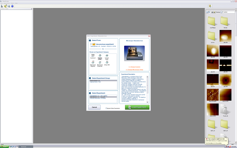
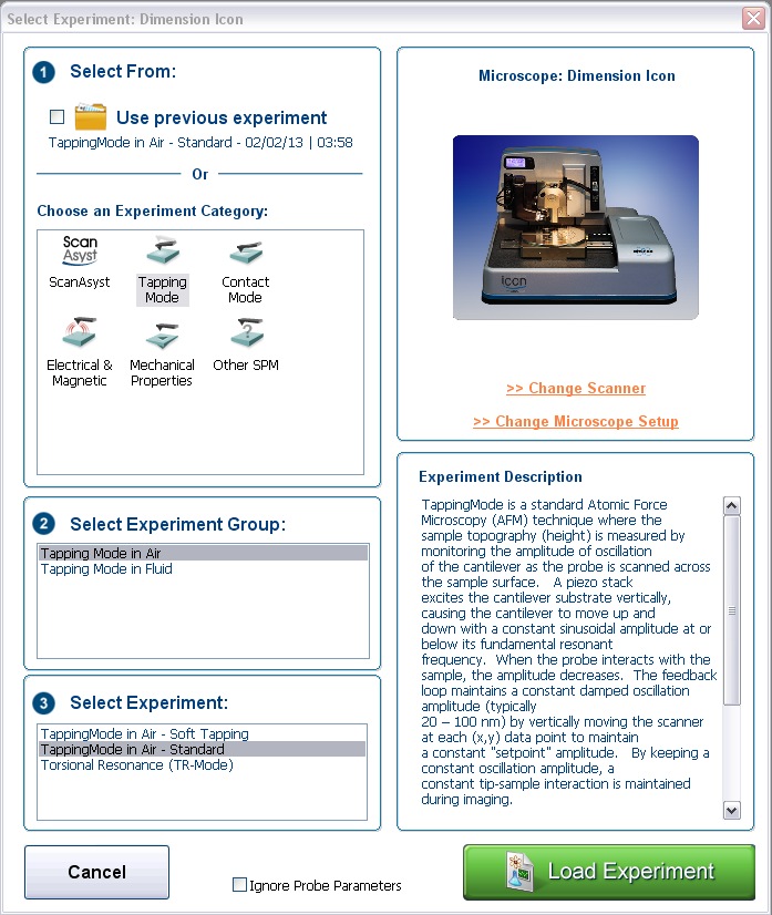
There are several Experiment Categories, each category has several groups
and each group has several experiments.
There is a quite extensive description for each experiment
that pops up to the right when that particular experiment is selected.
Click on Load Experiment to activate your selection. |
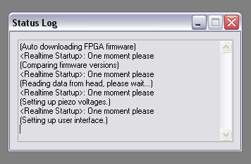
| When the experiment is loading, there is a start up procedure between the computer and the controller, there is a Status Log popping up showing the progress. |
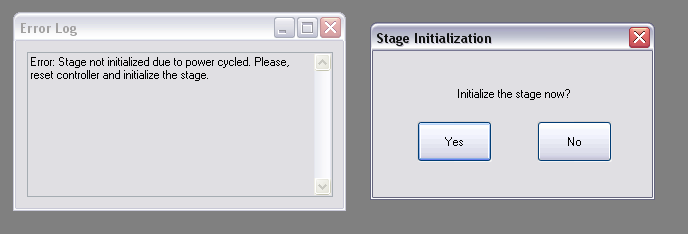
| If the ICON system was powered down when you start (most common) you will always get Stage Initialisation, you should answer Yes. |
|
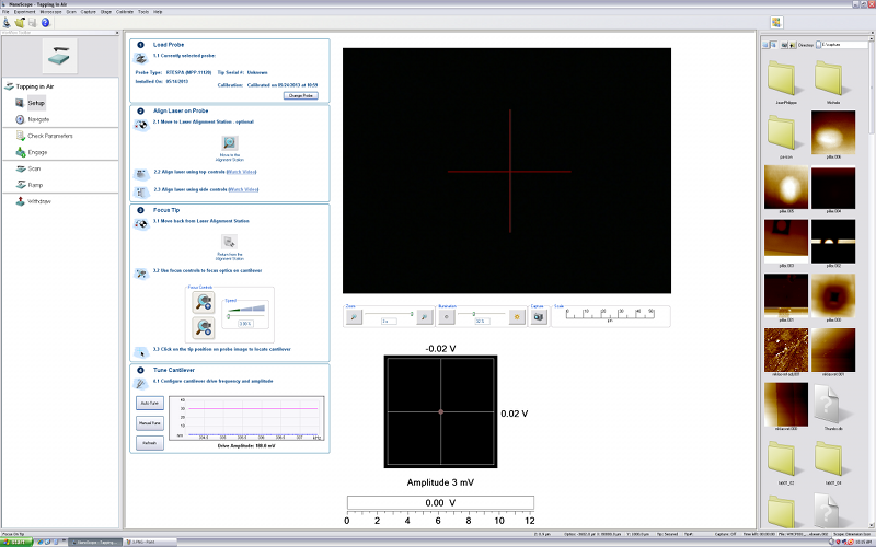
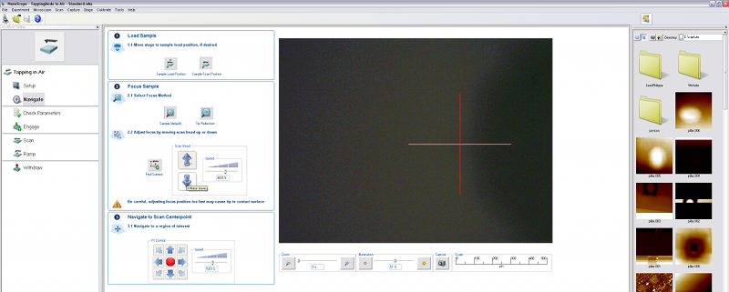
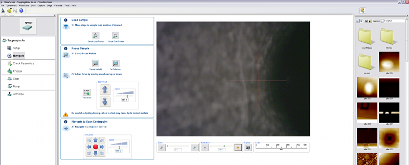
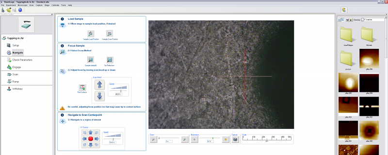
Here is the main page for the experiment. To the left is a column of
steps you must go through in order to start the scanning.
In the center frame are the steps to do the setup prior to scanning, the image area for the camera (now black) with a red cross that will indicate the tip position. Below are the indicators for the laser signal from the quad detector showing the position of the laser spot, below is the sum signal meter. At the far right is a column of icons of the contents for the currently selected image folder. Note that this is not necessarily the same as the folder where the scanned images are stored. |
|
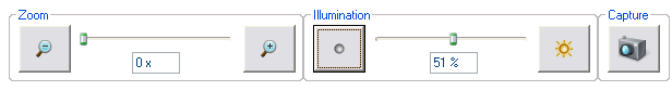
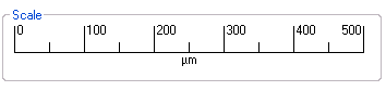
Here are the controls for the camera, right under the black image
field in the previous picture.
There is a Zoom control, only digital zoom in the 5 mega pixel image. Next is Illumination intensity control. Please note that if the scan head is too far away from the sample surface, the light might not be enough even at max intensity. This depends also on the reflectivity of the sample surface. If the scan head, i.e. the cantilever is within 5 mm of the surface, the light is usually enough. There is a Capture button to store the camera image on disk. At last there is a Scale following the setting of the zoom control. |
|
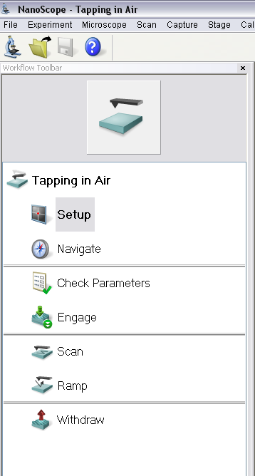
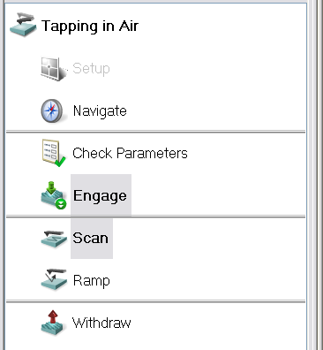
Here are the steps for the whole experiment.
Setup to align laser spot onto the quad detector, focus the tip and tune the cantilever. Navigate to focus the sample surface and locate the interesting part of the sample. Check Parameters to eventually tweak the parameter settings prior to scanning. Usually the default settings work very well. Engage to approach the surface and start scanning. Scan ?????? Ramp to collect force curves etc. Withdraw to end scanning and lift tip off the sample surface, in order to move to another part of the sample, switch samples or end the session. |
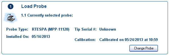
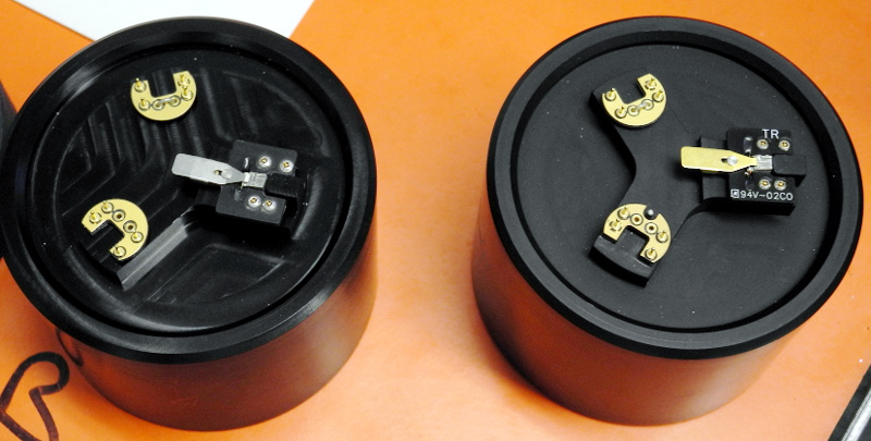
| Tell the software which probe (cantilever/tip) is mounted. Either a type number of a Bruker probe, or you can give data for some other make of probe. |
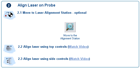
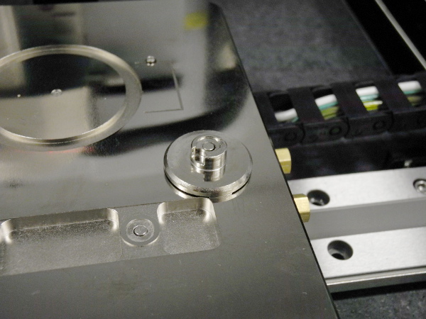
| Align laser spot on backside of cantilever. Use the position indicators and sum signal meter shown above. You can either observe the laser spot on the stage base (picture above) or move to the Alignment Station, a special position on the stage where the reflected laser spot can be seen in the camera image. |
|
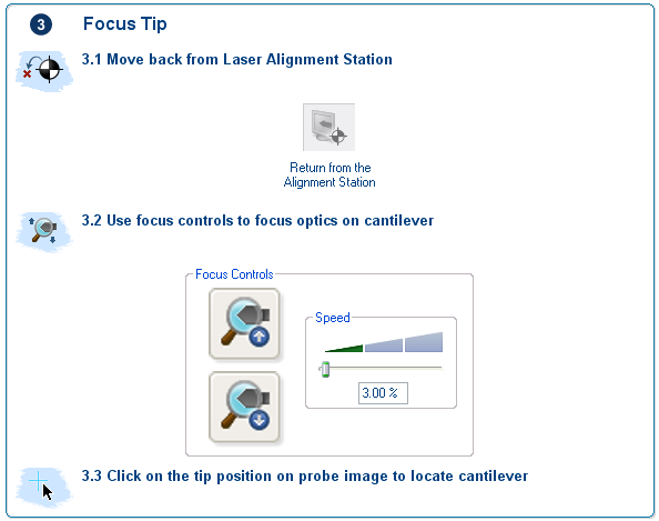
Focus Tip is very important. This tells the software
where the tip is
relative to the sample surface (see further below,
Focus Surface). In this way the software can move the
tip with high speed quite close to the surface without crashing the
tip. This saves time during Engage.
You have to move away from the Alignment Station on to the sample surface. In order to have enough light to see the tip you must be some millimeters from the sample surface, you may have to switch to Navigate to lower the scan head enough to make the cantilever visible. Use the Focus Controls to make the image as sharp as possible. You also click in the camera image to indicate where the tip is located on the cantilever, the red cross will move to that position (3.3 Click on ...). |
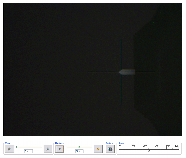
| This is how it should look when the tip/cantilever is on focus and the tip position is correctly indicated (red cross). |
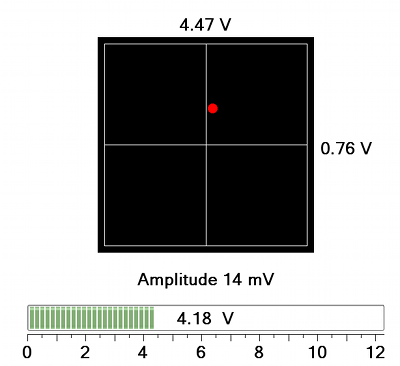
| Here are the indicators for the laser spot position on the quad detector. Note that it is not centered. The tapping amplitude is 14 mV and the sum signal is 4.18 V which is maximum in this case, for this particular cantilever. |
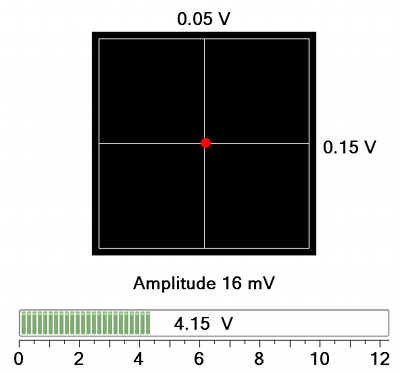
| Here the laser spot is centered on the quad detector using the knobs on the side of the scan head (the top knobs are for aligning laser spot onto the cantilever). The tapping amplitude and the sum signal changed a little, no further adjustment necessary. |
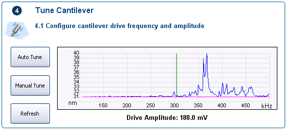
| For tapping mode you have to tune the cantilever to find the resonant frequency, and set the drive frequency. This is fully automatic in most cases. Click on Auto Tune to start. |
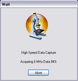
| The controller is acquiring data, both from a frequency sweep and from thermal calibration. |
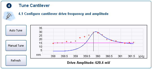
| Tuning is finished. Blue line is data from the frequency sweep, the small red crosses are from the thermal calibration, drive frequency is set to 359.8 kHz (vertical green line). |
| There is some light coming into the camera, you can see the unsharp contour of the cantilever. This means that the stage is moved to the approximate sample location and that the scan head (cantilever) is close enough to the sample (about 5 mm). |
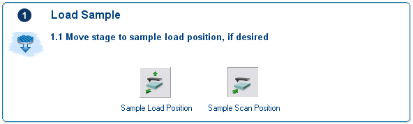
|
Sample Load Position means the stage moved forward for
easy access to the stage.
Sample Scan Position is undefined if you started the session by powering on the system. I.e. there is no "memory" of the previous users scan position if the system has been shut off.
Usually you use the stage controls (the roller ball unit or the
navigate controls, see below) to move the stage to the desired sample
position.
|
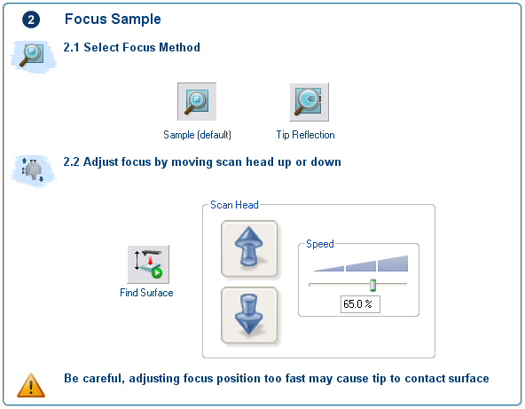
| Find the sample surface by getting a sharp image from the camera. | ||
| Focus Method: | Sample (default) means moving down the scan head until you see the sample surface in sharp focus. This can be difficult if the sample is very clean (no dust particles to see) or if the sample is very transparent (you see the underlying surface sharply and think you see the sample surface, you may crash the tip if sample is thick enough). | Tip Reflection: The scan head is moved down until you see the mirror image of the cantilever/tip sharply in the camera. |
|
The button Find Surface should be used cautiously, you
must be sure that the surface is easily found. You should know that
the surface either has a clear structure or sufficiently with
particles on it to be easily discovered.
Please notice the warning about speed of focus. |
||
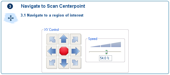
|
Use this control or the roller ball unit to move stage to desired
sample scan position.
NOTE! If you use the magnetic puck holder, take care so the scan head is high enough to not smash the cantilever sideways into the puck holder when moving the stage. |
|
Here the sample surface can be seen, although it is still
unsharp. Note that the cantilever is completely out of focus, the
camera focus is set for finding the surface.
Note! The only time the surface and the cantilever/tip are in focus together is during scanning. If this happens during focusing the surface there is a serious risk of crashing the tip. |
| Here the surface is in good focus. You can fine tune the stage position to find the best place to scan. |
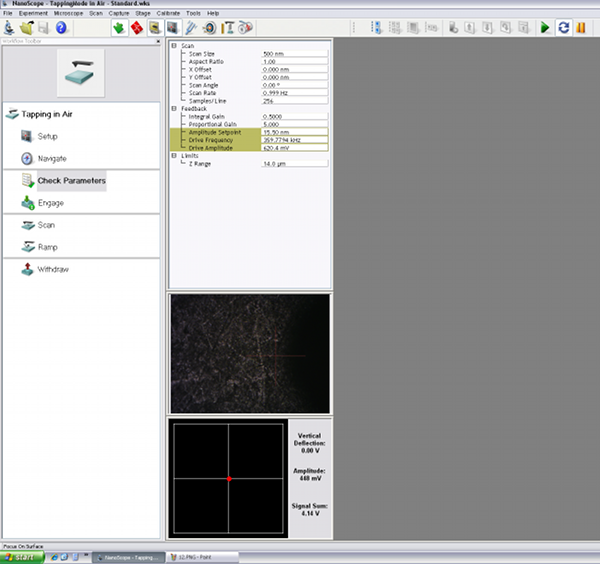
| Moving on the next step Check Parameters. The parameters for this experiment (standard tapping in air) are shown in the center. Below are displayed the camera image and the laser spot on quad sensor. |
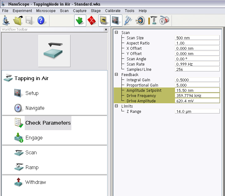
| Usually the default parameters are good for initial scanning. If the sample surface is very smooth, the Z Range may have to be decreased to increase the resolution in Z direction. Otherwise the height curve can have a staircase appearance. |
| Next click Engage. |
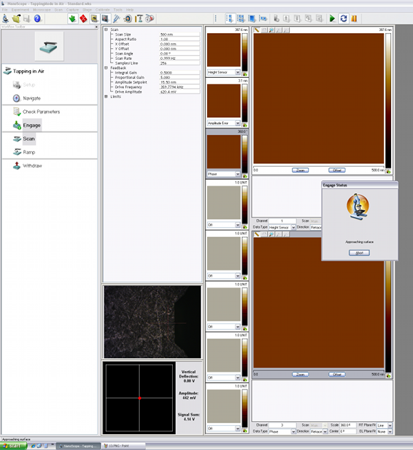
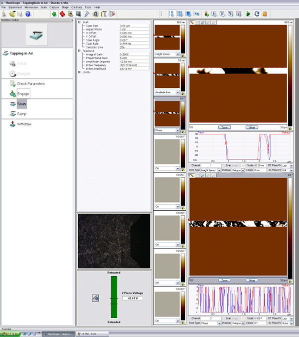
| The window layout during approach. Two of the three active signal channels are displayed to the right. It is possible to capture up to eight different signals. In this standard tapping mode only three are collected by default. |
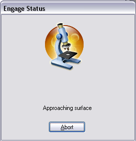
| The scan head is moving down, approaching the surface. |
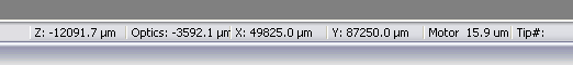
| During the approach the stepping motor position can be seen at the lower right part of the window (info bar). Here the absolute positions of the scan head (Z:), the optics, the stage are displayed. The last parameter Motor: is increasing as the approach is done, usually 80 - 100 µm is needed to make contact. |
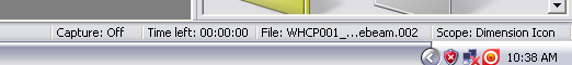
| The rightmost part of the info bar, the state of the image Capture flag, the capture file-name are important parameters. |
| Here the approach is finished and the scanning is started, collecting the first image data. |
|
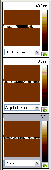
The scanning has started, collecting and displaying data in the three
channels:
Height Sensor which is the signal from the Z piezo position sensor. This is slightly different from the Height signal which is the voltage applied to the Z-piezo re-calculated to height via calibration data. Amplitude Error which is the error signal from the feedback loop trying to keep the cantilever at a constant height over the topography of the surface. Phase which is the phase lag between the drive signal and the signal from the laser-spot vibrating over the quad detector. |
|
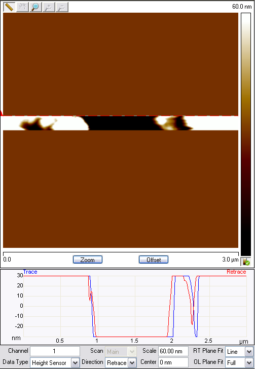
The window showing the Height Sensor data in full
resolution. The scan range has been increased to 3 µm from the
initial setting of 500 nm.
Below is shown the line profile for Trace and Retrace. Below the line profiles are settings for data collection for this channel, in this case the Retrace signal is used to build the image, the height display scale is limited to 60 nm, the Real Time Plane Fit is active on a line-by-line basis and the Off Line Plane Fit is fully active. NOTE! The Off Line Plane Fit affects the stored data, the captured file. To have the most control over the image, it is better to set the Off Line Plane Fit to Off or None, and do the plane fitting after the image has been captured. |
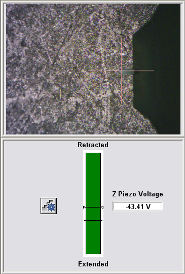
| The tip can be seen moving over the surface during scanning if the scan range is large enough. The position of the Z-piezo can be seen below the camera image. If the Z-piezo is getting fully Retracted or Extended it can be adjusted with the motor button to the left. This will move the step motor in small increments to get the Z-piezo within the normal working range. |
Specifications
Vibration specification
| X-Y scan range | 90µm x 90µm typical, 85µm minimum |
| Z range | 10µm typical in imaging and force curve modes, 9.5µm minimum |
| Vertical noise floor | <30pm RMS in appropriate environment typical imaging bandwidth (up to 625Hz) |
| X-Y position noise (closed-loop) | ≤0.15nm RMS typical imaging bandwidth (up to 625Hz) |
| X-Y position noise (open-loop) | ≤0.10nm RMS typical imaging bandwidth (up to 625Hz) |
| Z sensor noise level (closed-loop) | 35pm RMS typical imaging bandwidth (up to 625Hz); 50pm RMS, force curve bandwidth (0.1Hz to 5kHz) |
| Integral nonlinearity (X-Y-Z) | <0.5% typical |
| Sample size/holder | 210mm vacuum chuck for samples, ≤210mm diameter, ≤15mm thick |
|
Motorized position stage (X-Y axis) | 180mm × 150mm inspectable area; 2µm repeatability, unidirectional; 3µm repeatability, bidirectional |
| Microscope optics | 5-megapixel digital camera;
180µm to 1465µm viewing area; Digital zoom and motorized focus |
| Controller | NanoScope V |
| Workstation | Integrates all controllers and provides ergonomic design with immediate physical and visual access |
| Vibration isolation | Integrated, pneumatic |
| Acoustic isolation | Operational in environments with up to 85dBC continuous acoustic noise |
| AFM modes | Standard: ScanAsyst, TappingMode (air), Contact Mode, Lateral Force Microscopy, PhaseImaging, Lift Mode, MFM, Force Spectroscopy, PeakForce Tuna, Force Volume, EFM, Surface Potential, Piezoresponse Microscopy, Force Spectroscopy; Optional: PeakForce QNM, HarmoniX, Nanoindentation, Nanomanipulation, Nanolithograpy, Force Modulation (air/fluid), TappingMode (fluid), Torsional Resonance Mode, Dark Lift, STM, SCM, C-AFM, SSRM, TUNA, TR-TUNA, VITA |